Geometric Programming vs. Linear Programming for Metabolic Optimization: A Strategic Guide for Biomedical Researchers
This article provides a comprehensive comparison of Geometric Programming (GP) and Linear Programming (LP) for optimizing metabolic systems in biomedical research and drug development.
Geometric Programming vs. Linear Programming for Metabolic Optimization: A Strategic Guide for Biomedical Researchers
Abstract
This article provides a comprehensive comparison of Geometric Programming (GP) and Linear Programming (LP) for optimizing metabolic systems in biomedical research and drug development. It explores the foundational principles of both optimization frameworks, detailing their specific methodologies and applications in modeling metabolic pathways, dynamic regulation, and strain design. The content addresses critical troubleshooting aspects and performance optimization for each method, culminating in a validated, comparative analysis of their efficiency, accuracy, and applicability to real-world biological problems. Aimed at researchers and scientists, this guide synthesizes key insights to inform the selection and implementation of the most suitable optimization strategy for advanced metabolic engineering projects.
Core Principles: Unpacking the Mathematical Foundations of GP and LP in Biology
Linear Programming (LP) represents a cornerstone method in optimization, achieving the best outcome against a linear objective function within a constrained linear system [1]. Its application spans from logistics to metabolic engineering, where it provides a robust framework for flux balance analysis in biochemical networks [2]. However, biological systems often exhibit inherent nonlinearities that challenge LP's fundamental assumptions. This limitation has prompted the development of advanced optimization techniques, notably Geometric Programming (GP), which leverages the special structure of power-law models to efficiently solve nonconvex optimization problems prevalent in metabolic pathway engineering [3] [4]. While LP remains invaluable for stoichiometric models lacking regulatory details, GP has demonstrated superior performance in identifying global optima for nonlinear biochemical systems, achieving computational efficiency that positions it as a transformative methodology for complex metabolic optimization tasks [3] [4].
Fundamental Principles and Mathematical Foundations
Linear Programming: Core Formulations
Linear programming optimizes a linear objective function subject to linear equality and inequality constraints, with the standard form expressed as [1]: [ \text{Maximize } \mathbf{c}^T\mathbf{x} \quad \text{subject to} \quad A\mathbf{x} \leq \mathbf{b} \ \text{and} \ \mathbf{x} \geq \mathbf{0} ] Here, ( \mathbf{x} ) represents the decision variables, ( \mathbf{c} ) contains coefficients for the linear objective function, and ( A\mathbf{x} \leq \mathbf{b} ) defines the system constraints [1]. The feasible region formed by these constraints constitutes a convex polytope, with optimal solutions invariably located at corner points of this region [1].
The simplex algorithm, developed by George Dantzig in 1947, efficiently navigates these corner points to locate optima, while interior-point methods developed later provide polynomial-time solutions [1]. LP's computational efficiency enables solution of large-scale problems—Dantzig's original example of assigning 70 people to 70 jobs would have required checking more configurations than particles in the observable universe through enumeration, yet the simplex method finds the optimum in moments [1].
Geometric Programming: Extending to Nonlinear Domains
Geometric programming addresses a class of nonlinear optimization problems that can be transformed into convex forms through logarithmic/variable transformations [4]. GP specializes in optimizing posynomials—functions comprising sums of power-law terms (monomials) with positive coefficients [3] [4].
The GP standard form appears as: [ \text{Minimize } f0(\mathbf{x}) \quad \text{subject to} \quad fi(\mathbf{x}) \leq 1, \quad hj(\mathbf{x}) = 1 ] where ( fi ) are posynomials and ( h_j ) are monomials [4]. This structure proves particularly adept at handling Generalized Mass Action (GMA) systems in biochemical modeling, where each power-law term constitutes a monomial [3] [4]. Through logarithmic transformation of variables and constraints, GP converts nonconvex problems into convex forms solvable with high efficiency—problems with 1000 variables and 10,000 constraints can be solved in under a minute on standard desktop computers [4].
Table 1: Core Mathematical Properties Comparison
| Property | Linear Programming (LP) | Geometric Programming (GP) |
|---|---|---|
| Objective Function | Linear: ( \mathbf{c}^T\mathbf{x} ) | Posynomial: ( \sumk ck x1^{a{1k}} \cdots xn^{a{nk}} ) |
| Constraints | Linear inequalities/equalities | Posynomial inequalities, monomial equalities |
| Feasible Region | Convex polytope | Convex after logarithmic transformation |
| Variable Domain | Typically ( \mathbf{x} \geq \mathbf{0} ) | ( \mathbf{x} > \mathbf{0} ) |
| Solution Space | Corner points of polytope | Interior and boundary points after transformation |
| Global Optimality | Guaranteed for convex feasible region | Guaranteed after convex transformation |
Applications in Metabolic Optimization: A Comparative Analysis
Linear Programming in Metabolic Engineering
LP has established fundamental utility in metabolic engineering through Flux Balance Analysis (FBA), which predicts metabolic fluxes by assuming steady-state operation and mass balance constraints [2]. The key advantage lies in LP's computational efficiency with minimal information requirements—primarily flux rates and physico-chemical constraints [3]. This enables genome-scale modeling without demanding kinetic parameters [2].
Recent extensions integrate transcriptomic data through methods like Linear Programming based Gene Expression Model (LPM-GEM), which linearly embeds gene expression into FBA constraints to improve flux predictions across different nutritional conditions [2]. When validated against 13C tracer experiments, such LP-based approaches successfully predict carbon source utilization in Bacillus subtilis, demonstrating practical utility despite simplification of biological complexity [2].
Geometric Programming for Nonlinear Biochemical Systems
GP addresses fundamental limitations in LP approaches by directly capturing the nonlinear regulatory features of metabolic pathways through GMA systems within Biochemical Systems Theory (BST) [3] [4]. Unlike S-system representations that approximate multiple fluxes into aggregated power-laws, GMA models represent each enzymatic process separately as power-law functions, preserving biological fidelity [4].
The significance of GP extends beyond specialized applications—GMA systems contain stoichiometric, mass-action, and S-system models as special cases, while algebraic equivalence transformations can convert virtually any dynamical model into GMA form [3]. This universality, combined with GP's computational efficiency, enables global optimization of complex metabolic networks that evade LP's linearity constraints [3] [4].
Table 2: Metabolic Optimization Performance Metrics
| Performance Metric | Linear Programming | Geometric Programming |
|---|---|---|
| Computational Efficiency | Highly efficient for large-scale problems [1] | Efficient for nonlinear problems; solves 1000 variables in <1 minute [4] |
| Regulatory Representation | Cannot represent regulation [3] | Explicitly captures nonlinear regulation [3] |
| Steady-State Solution | Linear equations [3] | Nonlinear, converted to linear via log transformation [4] |
| Global Optimality | Guaranteed for linear models [1] | Guaranteed after convex transformation [4] |
| Model Type Compatibility | Stoichiometric models [3] | GMA, S-system, mass action models [3] |
| Tryptophan Biosynthesis Solution | Suboptimal [4] | Global optimum identified (>3× basal flux) [4] |
| Implementation Examples | LPM-GEM for B. subtilis carbon source prediction [2] | Anaerobic fermentation in S. cerevisiae; E. coli tryptophan operon [3] |
Experimental Protocols and Methodologies
LP Experimental Protocol: Gene Expression Integration
LPM-GEM Methodology [2]:
- Data Assembly: Collect microarray gene expression data and corresponding 13C metabolic flux data for validation
- Pre-processing: Map gene expression to proteins and reactions using Gene-Protein-Reaction (GPR) associations
- Model Construction:
- Transfer stoichiometric matrix, bounds, and reversibility from base metabolic model (e.g., iYO844 for B. subtilis)
- Implement three strategies to reduce thermodynamically infeasible loops
- Constraint Formulation: Embed continuous gene expression data linearly into FBA constraints
- Validation: Compare predicted fluxes against 13C tracer experimental data across multiple carbon source conditions
This protocol successfully predicted carbon sources for B. subtilis with accuracy outperforming established methods, demonstrating LP's practical utility despite its mathematical simplification of biological processes [2].
GP Experimental Protocol: Steady-State Optimization
Geometric Programming for GMA Systems [3] [4]:
- System Representation: Convert metabolic pathway to GMA formalism where each reaction rate ( vi ) follows power-law representation: [ vi = \gammai \prod{j=1}^{n+m} Xj^{f{i,j}} ] where ( \gammai ) is the rate constant and ( f{i,j} ) are kinetic orders [3]
Steady-State Formulation: Apply steady-state conditions ( \frac{dXi}{dt} = \sum \mu{ij} v_j = 0 ), resulting in system of monomial and posynomial equations [4]
Equivalence Transformation: Convert nonconvex GMA equations to GP-compatible form through:
- Variable substitution (( yi = \ln Xi ))
- Monomial condensation for posynomial constraints [4]
Geometric Programming Implementation:
- Solve transformed convex optimization problem
- Iteratively refine solution through sequential GP approximations
- Validate stability through eigenvalue analysis [5]
Bi-objective Extension: For multi-objective optimization (e.g., maximize product yield while minimizing metabolite concentrations):
- Apply Normal-Boundary Intersection (NBI) method
- Transform to single-objective optimization
- Generate Pareto optimal fronts [5]
This protocol has demonstrated superior performance in benchmark studies, including anaerobic fermentation in S. cerevisiae and tryptophan biosynthesis in E. coli, consistently identifying global optima that eluded previous optimization methods [3] [4].
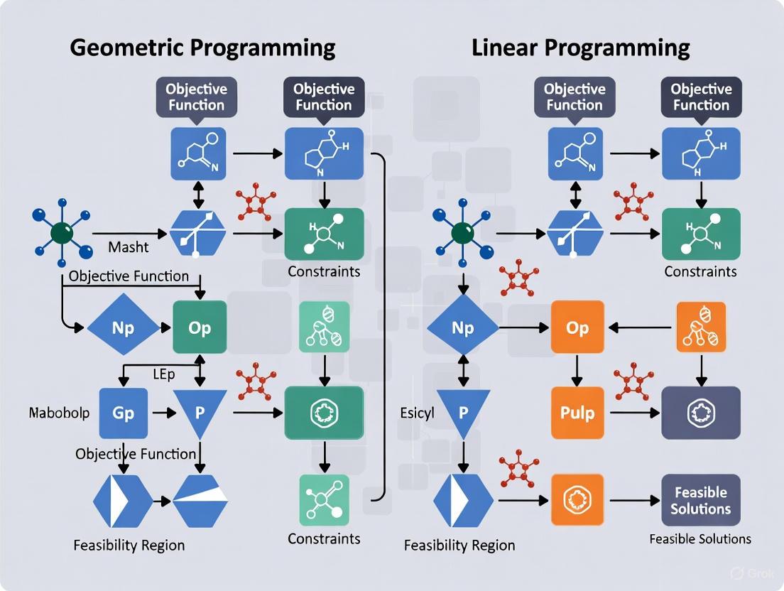
Figure 1: Comparative Methodological Workflows for LP and GP in Metabolic Optimization
Table 3: Essential Research Tools for Metabolic Optimization Studies
| Tool/Resource | Function/Purpose | Compatibility |
|---|---|---|
| GGPLAB | MATLAB-based GP solver for biochemical systems [4] | Geometric Programming |
| Gurobi Optimizer | Commercial solver for LP and related problems [6] | Linear Programming |
| BiGG Models Database | Curated metabolic models (e.g., iYO844 for B. subtilis) [2] | Both LP and GP approaches |
| Gene-Protein-Reaction (GPR) Mapping | Links gene expression to metabolic reactions [2] | Both LP and GP approaches |
| 13C Tracer Flux Data | Gold standard validation for predicted metabolic fluxes [2] | Both LP and GP approaches |
| Normal-Boundary Intersection (NBI) | Method for multi-objective optimization [5] | Primarily GP |
| BST-Based Modeling Tools | Biochemical Systems Theory implementation for GMA models [3] | Geometric Programming |
Critical Analysis and Research Outlook
The comparative analysis reveals a complementary relationship between LP and GP in metabolic optimization. LP maintains advantages in computational efficiency and implementation simplicity for large-scale stoichiometric models, particularly when integrated with transcriptomic data through methods like LPM-GEM [2]. However, GP demonstrates unequivocal superiority for problems requiring accurate representation of nonlinear regulatory dynamics, achieving global optima that escape LP-based methods [3] [4].
Recent advances address GP's historical limitations through improved handling of nonconvex problems via equivalence transformation and monomial compensation strategies [4]. For S-type biochemical systems, GP successfully solves nonconvex bi-objective optimization problems with stability guarantees, generating Pareto optimal solutions that balance product yield maximization with metabolite concentration minimization [5].
Future research trajectories include hybrid approaches leveraging LP's scalability for initial screening and GP's precision for refined optimization of promising metabolic engineering targets. The integration of thermodynamic constraints with geometric programming represents another fruitful direction, potentially bridging the gap between thermodynamic feasibility and regulatory complexity in metabolic models [2].
For researchers selecting between these methodologies, the decision framework should prioritize LP when working with genome-scale stoichiometric models lacking detailed kinetic information, and GP when optimizing well-characterized pathways with known regulatory interactions and nonlinear dynamics. As kinetic modeling advances through improved parameter estimation, GP's strategic importance in metabolic engineering will likely expand, establishing it as the methodology of choice for precision optimization of complex biochemical systems.
Geometric Programming (GP) represents a powerful class of constrained nonlinear optimization problems that has found significant application in metabolic engineering and systems biology. Unlike generic nonlinear optimization, GP possesses unique mathematical properties that enable efficient solution of otherwise computationally challenging problems. When applied to metabolic optimization, GP allows researchers to manipulate metabolic networks to improve desired characteristics of biochemical systems, such as maximizing product yield or redirecting metabolic flux toward valuable compounds [7].
The fundamental advantage of GP in biological contexts stems from its ability to model the highly nonlinear nature of biochemical processes while maintaining computational tractability. This is particularly valuable in metabolic engineering tasks where the goal is to identify optimal genetic manipulations or process conditions that maximize the production of target metabolites while maintaining cellular viability and function [7] [4]. The comparison between GP and linear programming (LP) approaches is especially relevant because many traditional metabolic optimization methods rely on linear approximations of biological systems, which may fail to capture essential nonlinear dynamics.
Mathematical Foundations of Geometric Programming
Core Components: Monomials and Posynomials
The mathematical structure of GP is built upon two special types of functions: monomials and posynomials. Understanding these components is essential for formulating problems within the GP framework.
A monomial is defined as a function of the form:
[f(x) = c x1^{a1} x2^{a2} ... xn^{an}]
where:
- (c) is a positive constant
- (x_{1..n}) are positive decision variables
- (a_{1..n}) are real exponents [8]
Examples of monomials include (7x), (4xy^2z), and (\frac{2x}{y^2z^{0.3}}) [8]. In the context of biochemical systems, monomials naturally represent kinetic rate laws, enzyme-catalyzed reactions, and other fundamental biological processes [7].
A posynomial extends this concept as a sum of monomials:
[g(x) = \sum{k=1}^K ck x1^{a1k} x2^{a2k} ... xn^{ank}]
Examples of posynomials include expressions like (x^2 + 2xy + 1) and (7xy + 0.4(yz)^{-1/3}) [8]. In metabolic modeling, posynomials can represent aggregated biological processes, such as the combined activity of multiple enzymatic pathways or the total flux through branched metabolic networks [7].
The Convex Transformation
The remarkable property of GP that distinguishes it from general nonlinear optimization is its transformability to a convex optimization problem. This transformation occurs through a logarithmic change of variables that converts the inherently nonconvex GP into a convex form, guaranteeing that any local optimum is also globally optimal [8].
The transformation process works as follows:
- Original variables (xi > 0) are replaced with their logarithms: (yi = \log x_i)
- Monomials become linear functions in the new variables: (c \prod xi^{ai} = c \exp(\sum ai yi))
- Posynomials become log-sum-exp functions, which are convex [9]
This convex transformation enables GP problems to be solved "extremely quickly" and "with no initial guesses or tuning of solver parameters" [8]. For perspective, "a GP with 1000 variables and 10,000 constraints can be solved in under a minute on a desktop computer" [4].
The following diagram illustrates this convex transformation process:
GP vs. LP: Methodological Comparison for Metabolic Optimization
Fundamental Differences in Problem Formulation
While both Geometric Programming and Linear Programming are used for metabolic optimization, they differ fundamentally in their mathematical structure and biological representation.
Linear Programming (LP) in Metabolism:
- Represents metabolic networks using stoichiometric matrices [10]
- Assumes steady-state operation with constant metabolite concentrations [10]
- Optimizes flux distributions through linear constraints [11]
- Cannot directly represent regulatory features or nonlinear kinetics [7]
Geometric Programming (GP) in Metabolism:
- Represents metabolic processes using power-law functions within Generalized Mass Action (GMA) systems [7] [4]
- Can capture nonlinear enzyme kinetics and regulatory interactions [7]
- Maintains mathematical tractability through convex transformation [8]
- Allows optimization of both metabolic fluxes and enzyme activities [4]
The key advantage of GP lies in its ability to model the inherent nonlinearity of biological systems while maintaining computational efficiency. As one study notes, "GMA systems are of importance because they contain stoichiometric, mass action and S-systems as special cases" [7], making them a more comprehensive framework for biological optimization.
Application to Metabolic Network Optimization
The practical differences between GP and LP approaches become evident when applied to specific metabolic optimization tasks. The following table summarizes their comparative performance based on experimental studies:
Table 1: Comparative Performance of GP vs. LP in Metabolic Optimization
| Aspect | Geometric Programming (GP) | Linear Programming (LP) |
|---|---|---|
| Mathematical Foundation | Power-law functions in GMA systems [7] | Linear stoichiometric models [10] |
| Regulatory Representation | Can directly represent enzyme regulation and inhibition [7] | Cannot capture regulatory features [7] |
| Solution Efficiency | Solves nonconvex problems through convex transformation [4] | Efficient for linear problems but limited in nonlinear contexts [11] |
| Optimality Guarantee | Global optimum guaranteed for transformed problem [8] | Global optimum for linear formulation only [11] |
| Implementation Example | Optimization of anaerobic fermentation in S. cerevisiae [7] | Flux Balance Analysis (FBA) in E. coli models [10] |
Experimental Protocols and Case Studies
Protocol for GP-Based Metabolic Optimization
Implementing geometric programming for metabolic optimization involves a systematic procedure that leverages the special structure of GMA systems:
Model Formulation: Represent the metabolic network as a GMA system where each reaction rate follows power-law formalism: [vi = \gammai \prod{j=1}^{n+m} Xj^{f{i,j}}] where (\gammai) is the rate constant, (Xj) are metabolic concentrations, and (f{i,j}) are kinetic orders [7].
Steady-State Establishment: Define the steady-state constraints using the stoichiometric matrix (N) and flux vector (v): [\frac{dX}{dt} = N \cdot v = 0] which ensures mass balance within the metabolic network [7].
Objective Function Specification: Formulate the optimization target (e.g., product yield maximization) as a posynomial function of the system variables [4].
Constraint Definition: Include additional posynomial constraints representing physical, metabolic, and physiological limitations [7].
Convex Transformation: Apply logarithmic transformation to convert the GP to a convex optimization problem [8].
Solution Implementation: Solve the transformed problem using GP solvers such as GGPLAB [4] or CVXPY with DGP capabilities [9].
The following workflow diagram illustrates this experimental protocol:
Case Study: Tryptophan Biosynthesis Optimization
A comparative study optimizing tryptophan biosynthesis in E. coli demonstrated the advantages of GP over alternative methods. The GP approach successfully identified the global optimal solution that maximized tryptophan flux, achieving more than 3 times the basal flux [4]. This performance exceeded that of controlled error and penalty treatment methods, which failed to reach the global optimum in the same problem [4].
The successful application of GP to this system highlights its practical value for metabolic engineering, where identifying true optimal solutions can significantly impact production yields in industrial biotechnology.
Case Study: Anaerobic Fermentation Pathway Optimization
Another benchmark study applied GP to optimize the anaerobic fermentation pathway in S. cerevisiae [7]. The GP formulation efficiently handled the nonlinear kinetics of the fermentation pathway and identified optimal manipulation strategies for yield improvement. The method demonstrated equal or better performance compared to earlier optimization approaches "in terms of successful identification of optima and efficiency" [7].
Implementing geometric programming for metabolic optimization requires specific computational tools and resources. The following table outlines key components of the research toolkit:
Table 2: Essential Research Reagents and Computational Tools for GP-Based Metabolic Optimization
| Tool/Resource | Type | Function in GP Metabolic Optimization |
|---|---|---|
| GMA Models | Mathematical Framework | Represents metabolic networks with power-law functions for GP compatibility [7] |
| CVXPY with DGP | Software Library | Python-embedded modeling language for disciplined geometric programming [9] |
| GGPLAB | GP Solver | MATLAB-based solver for geometric programming problems [4] |
| S-system Models | Special Case | Simplified BST representation convertible to GP form [7] |
| Biochemical Systems Theory (BST) | Theoretical Framework | Provides foundation for power-law modeling of biological systems [7] |
| Flux Balance Analysis | Complementary Method | Provides constraint information for GP metabolic models [10] |
Geometric Programming provides a mathematically rigorous and computationally efficient framework for metabolic optimization that surpasses linear programming approaches in handling biological nonlinearity. Through its foundation in monomial and posynomial functions and the powerful convex transformation, GP enables researchers to identify globally optimal solutions to complex metabolic engineering problems.
The experimental evidence from case studies on tryptophan biosynthesis and anaerobic fermentation pathways demonstrates that GP consistently outperforms traditional optimization methods, including LP-based approaches, in both solution quality and computational efficiency. As metabolic engineering continues to address increasingly complex biological systems, Geometric Programming offers a versatile and powerful approach for unlocking the full potential of cellular metabolism for biomedical and biotechnological applications.
Metabolic network modeling represents a cornerstone of systems biology, enabling the prediction of cellular behavior and the identification of strategic interventions for biotechnological and therapeutic applications. The core challenge lies in selecting and executing the appropriate computational strategy to manipulate these complex biochemical systems effectively. Optimization techniques provide the mathematical foundation for navigating these high-dimensional spaces, with linear programming (LP) and geometric programming (GP) emerging as two powerful, yet philosophically and technically distinct, paradigms. While LP has long been a staple in constraint-based modeling due to its simplicity and reliability, GP offers a sophisticated framework for tackling the inherent nonlinearities of metabolic kinetics. This guide provides a structured comparison of these two approaches, detailing their theoretical underpinnings, practical applications, and performance characteristics to inform their use in metabolic engineering and drug development research.
Theoretical Foundations: A Tale of Two Frameworks
The distinction between Linear Programming and Geometric Programming begins at the most fundamental level of mathematical representation and problem formulation.
Linear Programming (LP) in Metabolism: LP is applied to metabolic networks whose steady-state behavior can be described using systems of linear equations. This is most commonly achieved through Stoichiometric Models, such as those used in Flux Balance Analysis (FBA), where the mass-balance constraint at steady state (
Nv = 0) creates a linear system [3] [12]. A key innovation was the application of Biochemical Systems Theory (BST), which allows nonlinear kinetic models to be recast into a simplified power-law representation known as an S-system. When expressed in logarithmic coordinates, the steady-state equations of an S-system become linear, enabling the use of efficient LP algorithms for optimization [3] [13]. The objective function and all constraints in an LP problem are linear combinations of the decision variables.Geometric Programming (GP) in Metabolism: GP, in contrast, is a specialized nonlinear optimization technique that is exceptionally well-suited for models whose dynamics are inherently nonlinear. It is the natural framework for optimizing General Mass Action (GMA) systems within BST [3]. A GMA system represents each reaction rate as a monomial (a single power-law term), and the system dynamics are described by a sum of such monomials. The standard form of a GP requires the objective function and constraints to be posynomials (sums of monomials with positive coefficients) [3]. After a logarithmic transformation of variables, a GP can be converted into a convex optimization problem, guaranteeing the discovery of a global optimum.
Table 1: Core Mathematical Characteristics of LP and GP
| Feature | Linear Programming (LP) | Geometric Programming (GP) |
|---|---|---|
| Underlying Model | S-system (BST), Stoichiometric Model | GMA System (BST), Mass Action |
| Problem Formulation | Linear objective & constraints | Posynomial objective & constraints |
| Variable Transformation | Often uses logarithmic coordinates (for S-systems) | Logarithmic transformation to convex form |
| Solution Guarantee | Global optimum (for convex feasible region) | Global optimum (after transformation) |
| Mathematical Property | Linear | Nonlinear, but convex in log-space |
Performance Comparison: Quantitative Benchmarks
Experimental comparisons of LP and GP have been conducted on prototype metabolic networks and real-world pathways to evaluate their efficacy in solving bi-level optimization problems and identifying optimal steady states.
In one study, a bi-level optimization framework was deployed to maximize the final concentration of a target metabolite in a prototype network, where the product yield competes with cellular growth. The inner loop of this framework was solved using both LP and GP, and their performance was benchmarked against a direct optimization method that assumed full knowledge of the network kinetics. Both LP and GP successfully identified the optimal regulatory switch time (t_reg = 9s). However, the profile of the final product yield J(t_reg) was better approximated by the GP-based method, indicating a slight advantage in handling the network's nonlinear trade-offs [14].
Another significant application involves bi-objective optimization, where the goal is to maximize a desired product flux while simultaneously minimizing the total metabolite concentration (a proxy for metabolic burden). Research has shown that GP-based algorithms are highly effective at solving the nonconvex optimization models that arise from this problem, efficiently generating Pareto optimal fronts that illustrate the trade-off between the two competing objectives [5]. This capability is crucial for designing metabolically efficient cell factories.
Table 2: Experimental Performance Metrics for LP and GP
| Application Context | Optimization Method | Reported Outcome | Key Advantage |
|---|---|---|---|
| Bi-Level Optimization [14] | Linear Programming (LP) | Correctly identified optimal switch time (t_reg = 9s), good approximation of product yield. |
Reliability and computational speed. |
| Bi-Level Optimization [14] | Geometric Programming (GP) | Correctly identified optimal switch time (t_reg = 9s), slightly better yield profile than LP. |
Superior handling of nonlinear dynamics. |
| Bi-Objective Optimization [5] | Geometric Programming (GP) | Successfully solved nonconvex model, obtained Pareto optimal solutions. | Ability to find global optimum in complex trade-off spaces. |
| Steady-State Optimization [3] | Geometric Programming (GP) | Efficient optimization of GMA systems; equal or better than prior methods in identifying optima. | Versatility in directly optimizing nonlinear kinetic models. |
Experimental Protocols: From Model to Optimum
The practical application of LP and GP follows a structured workflow. Below is a detailed protocol for a typical bi-level optimization task, a common challenge in metabolic engineering.
Protocol: Bi-Level Optimization for Metabolite Overproduction
1. Problem Definition and Network Selection
- Objective: Maximize the final concentration of a target metabolite
x5at a fixed final timet_finalin a network where its production competes with biomass precursorx3. - Control Variable: Define
u(t)as the control input that redirects metabolic flux between the growth (v2) and production (v3) branches. The control is constrained to the interval[0, 1][14]. - Theoretical Insight: Using Pontryagin's Maximum Principle, it can be proven that the optimal control profile
u*(t)for such a network is bang-bang, meaning it only takes extreme values of 0 or 1, with at most one switching event [14].
2. Mathematical Model Formulation
- Implement the dynamic S-system or GMA model. For the prototype network, the equations are [14]:
dx1/dt = k - β1 * x1^h11dx2/dt = α2 * x1^g21 - β2 * x3^h23 * x2^h22dx3/dt = α3 * x2^g32 * (1 - u)dx4/dt = α4 * x3^g43 * x2^g42 * u - β4 * x4^h44dx5/dt = α5 * x4^g54 - Parameterization: Use known kinetic parameters (
α_i,β_i,g_ij,h_ij) and initial metabolite concentrationsx(0)[14].
3. Optimization Execution
- Direct Optimization (Benchmark): Use the full kinetic model to simulate the system for all possible switching times
t_regand identify the one that maximizesx5(t_final). This establishes the performance benchmark [14]. - Bi-Level Optimization with LP:
- Outer Loop: Iterate over possible switching times
t_reg. - Inner Loop (LP): For a candidate
t_reg, the problem is formulated as an S-system in logarithmic coordinates. A linear program is solved to find the flux distribution that maximizes product yield, subject to steady-state and capacity constraints [14] [13].
- Outer Loop: Iterate over possible switching times
- Bi-Level Optimization with GP:
4. Validation and Analysis
- Compare the optimal
t_regand the resultingx5(t_final)obtained from the LP and GP bi-level methods against the benchmark from direct optimization. - Analyze the metabolite time courses (e.g.,
x3andx5) for the optimal solution to understand the system's dynamic response.
Diagram 1: Workflow for comparing LP and GP in bi-level metabolic optimization.
Successful implementation of these optimization strategies relies on a combination of computational tools and theoretical frameworks.
Table 3: Essential Research Reagent Solutions for Metabolic Optimization
| Tool/Resource | Type | Function in Research |
|---|---|---|
| S-system Formalism [3] [13] | Modeling Framework | Represents nonlinear metabolic kinetics with power-law functions, enabling transformation into linear equations for LP at steady state. |
| GMA System Formalism [3] | Modeling Framework | Represents metabolic kinetics as a sum of monomials, forming the natural posynomial structure for GP optimization. |
| Biochemical Systems Theory (BST) [3] [13] | Theoretical Framework | Provides the foundation for both S-system and GMA representations, unifying the modeling of complex biochemical networks. |
| Flux Balance Analysis (FBA) [14] [12] | Computational Method | A foundational LP-based technique for predicting steady-state metabolic fluxes in genome-scale stoichiometric models. |
| OptiFold/Geometric Program Solver [3] | Software Tool | A specialized solver for geometric programming problems, capable of efficiently finding the global optimum for GMA system models. |
The choice between Linear Programming and Geometric Programming is not a matter of declaring one universally superior, but of matching the tool to the task. Linear Programming remains a highly efficient and robust choice for optimizing stoichiometric models and S-system approximations at steady state. Its strength lies in its computational speed and reliability for large-scale problems. Geometric Programming, while potentially more computationally intensive, offers a more direct and powerful framework for optimizing nonlinear kinetic models, such as GMA systems, often delivering marginally superior performance in capturing complex metabolic trade-offs.
Future research directions point toward greater integration and specialization. The development of hybrid models that leverage the scalability of LP for core metabolism and the precision of GP for regulated pathways holds great promise. Furthermore, the application of these techniques is expanding beyond single-objective strain design to complex areas such as understanding metabolic trade-offs in cancer [15] [16] and inferring context-specific cellular objectives from multi-omics data [12]. As metabolic models continue to grow in size and complexity, the complementary strengths of LP and GP will be crucial in translating computational predictions into real-world biotechnological and therapeutic breakthroughs.
Biochemical Systems Theory (BST) provides a powerful mathematical framework for modeling and analyzing complex biochemical networks. Its core innovation is the Power-Law Formalism, which uses power-law functions to represent the rate of biochemical processes through approximated, locally-linear models in logarithmic space [17]. This formalism is the simplest representation consistent with well-known growth laws and allometric relationships—the most regular, quantitative features observed among systemic variables in complex biochemical systems [18]. Within BST, two primary model representations have emerged: the Synergistic System (S-system) and the Generalized Mass Action (GMA) system. These representations form a critical bridge between biological reality and mathematical optimization, enabling the application of powerful optimization techniques like geometric and linear programming to metabolic engineering challenges.
The fundamental building block for both S-system and GMA representations is the power-law term. For a biochemical reaction rate ( vi ), this is formulated as ( vi = \alphai \prod{j=1}^{n} Xj^{g{ij}} ), where ( \alphai ) is the apparent rate constant and the exponent ( g{ij} ) is the apparent kinetic order [17]. These kinetic orders are local sensitivities in log space, defined as ( g{ij} = \frac{\partial vi}{\partial Xj} \frac{Xj}{vi} = \frac{\partial \log(vi)}{\partial \log(X_j)} ), making them exactly equivalent to the elasticities used in Metabolic Control Analysis [17]. This parameterization allows each model parameter to map uniquely onto structural and regulatory features of biological networks, providing biological interpretability that unstructured fitting models like high-order polynomials lack [19].
Mathematical Representations: S-system vs. GMA Formulations
S-system Representation
The S-system representation is characterized by its streamlined structure, where the net change in each dependent variable is represented by a single aggregate power-law function for production and another for degradation. For a system with ( n ) dependent variables, the S-system formulation is:
[ \frac{dXi}{dt} = \alphai \prod{j=1}^{n+m} Xj^{g{ij}} - \betai \prod{j=1}^{n+m} Xj^{h_{ij}} \quad (i = 1, 2, ..., n) ]
Here, ( \alphai ) and ( \betai ) are rate constants for production and degradation, respectively, while ( g{ij} ) and ( h{ij} ) are kinetic orders for production and degradation, respectively [3]. The first ( n ) variables are dependent, and the next ( m ) variables are independent (typically constant during simulations). This representation aggregates all production processes into one term and all degradation processes into another, resulting in a highly structured nonlinear system that nevertheless displays linear steady-state equations [3]. This linearity at steady state enables the application of linear programming methods for optimization tasks, a significant computational advantage.
GMA System Representation
In contrast to the S-system approach, the GMA representation maintains the identity of individual fluxes without aggregation. In this formulation, each reaction rate is represented as a separate power-law term, resulting in:
[ \frac{dXi}{dt} = \sum{k=1}^{pi} \gamma{ik} \prod{j=1}^{n+m} Xj^{f_{ijk}} \quad (i = 1, 2, ..., n) ]
where ( \gamma{ik} ) are rate constants and ( f{ijk} ) are kinetic orders for each specific reaction [3] [19]. The number of terms ( p_i ) can vary for each equation. GMA systems are particularly valuable because they contain both stoichiometric models and S-systems as special cases, allowing seamless transition from linear to fully kinetic models [19]. This representation is closer to biochemical intuition as production and degradation terms don't vanish if one contributing flux disappears, unlike in S-system aggregation [19].
Table 1: Comparison of S-system and GMA Representations
| Feature | S-system Representation | GMA Representation |
|---|---|---|
| Mathematical Form | One production & one degradation term per equation | Multiple terms per equation representing individual fluxes |
| Flux Aggregation | Aggregates all production/degradation fluxes | Maintains separate identity of each flux |
| Steady-State Properties | Linear equations at steady state | Nonlinear equations at steady state |
| Optimization Compatibility | Linear Programming (LP) | Geometric Programming (GP) |
| Biological Interpretation | Systemic perspective | Mechanistic, reaction-centric perspective |
| Parameter Estimation | More parameters per equation but fewer terms | More terms but direct mapping to reactions |
| Behavior if Flux Disappears | Entire aggregated term vanishes | Only the specific term disappears |
Optimization Methodologies: Geometric Programming vs. Linear Programming
Geometric Programming for GMA Systems
Geometric Programming (GP) is a powerful mathematical optimization tool that can be applied to problems where objective and constraint functions have a special form [14]. GP is particularly well-suited for optimizing GMA systems because the standard form of a GP problem consists of a posynomial objective function subject to posynomial constraints—a structure that naturally aligns with GMA equations [3]. A posynomial is a function of the form ( f(x) = \sum{k} ck x1^{a{1k}} x2^{a{2k}} \cdots xn^{a{nk}} ) where ( ck > 0 ) and ( a{ik} ) are real numbers, which matches the structure of GMA differential equations.
The advantage of GP in metabolic optimization lies in its ability to solve large-scale problems with extreme efficiency and reliability [14]. Even though GP problems are nonlinear, they can be transformed into convex optimization problems through a logarithmic transformation of variables, ensuring convergence to a global optimum [3]. This property is particularly valuable in metabolic engineering where local optima can lead to suboptimal strain designs. The application of GP to GMA systems has demonstrated equal or better performance compared to earlier methods in terms of successful identification of optima and efficiency [3].
Linear Programming for S-system Optimization
The S-system representation enables the application of Linear Programming (LP) for metabolic optimization by leveraging its linear steady-state equations. At steady state, where ( \frac{dX_i}{dt} = 0 ), the S-system equations become:
[ \alphai \prod{j=1}^{n+m} Xj^{g{ij}} = \betai \prod{j=1}^{n+m} Xj^{h{ij}} \quad (i = 1, 2, ..., n) ]
Taking logarithms of both sides transforms this product of power-laws into a system of linear equations [3]. This linearity enables the use of efficient LP algorithms for optimization tasks such as flux maximization or metabolite yield optimization. The transformation to linear equations occurs through defining new variables ( yi = \ln Xi ), which converts the power-law equations into:
[ \sum{j=1}^{n+m} (g{ij} - h{ij}) yj = \ln \betai - \ln \alphai ]
This linear structure allows metabolic optimization problems to be formulated with a linear objective function (e.g., maximizing biomass production or target metabolite yield) subject to linear constraints derived from the steady-state equations, along with additional linear constraints representing physicochemical limits and cellular viability requirements [3].
Table 2: Comparison of Optimization Methods for BST Representations
| Optimization Aspect | Geometric Programming (GMA) | Linear Programming (S-system) |
|---|---|---|
| Problem Type | Nonlinear but convertible to convex | Linear |
| Solution Guarantees | Global optimum guaranteed | Global optimum guaranteed |
| Computational Efficiency | Highly efficient for medium-large problems | Extremely efficient, scales to very large problems |
| Steady-State Requirement | Not required for dynamic optimization | Required for linearization |
| Implementation Complexity | Moderate | Low |
| Regulatory Constraints | Easily incorporated | Requires reformulation |
| Range of Applications | Dynamic and steady-state optimization | Primarily steady-state optimization |
Experimental Protocols and Case Studies
Prototype Network for Optimization Benchmarking
Researchers have developed a standardized prototype metabolic network to benchmark optimization strategies for BST representations [14]. This network represents a modified version of a previously established model and includes five metabolites with the following structure:
The differential equations for this system in GMA form are: [ \begin{align} \frac{dx_1}{dt} &= k - v_1 \ \frac{dx_2}{dt} &= v_1 - v_2(1-u) - v_3u \ \frac{dx_3}{dt} &= v_2(1-u) \ \frac{dx_4}{dt} &= v_3u - v_4 \ \frac{dx_5}{dt} &= v_4 \end{align} ]
where ( u ) represents a control function that redirects metabolic flux between branches leading to different products [14]. In S-system form, the same network is described as: [ \begin{align} \frac{dx_1}{dt} &= k - \beta_1 x_1^{h_{11}} \ \frac{dx_2}{dt} &= \alpha_2 x_1^{g_{21}} - \beta_2 x_3^{h_{23}} x_2^{h_{22}} \ \frac{dx_3}{dt} &= \alpha_3 x_2^{g_{32}} (1-u) \ \frac{dx_4}{dt} &= \alpha_4 x_3^{g_{43}} x_2^{g_{42}} u - \beta_4 x_4^{h_{44}} \ \frac{dx_5}{dt} &= \alpha_5 x_4^{g_{54}} \end{align} ]
This network exemplifies the classic trade-off in metabolic engineering where one metabolite (( x3 )) supports cell growth while another (( x5 )) represents the desired product, creating an optimization challenge to balance these competing objectives [14].
Figure 1: Prototype Metabolic Network with Competing Pathways
Optimization Workflow for Metabolic Pathways
The general optimization workflow for metabolic pathways using BST representations follows a systematic process that can be implemented through various computational frameworks:
Figure 2: BST-Based Metabolic Optimization Workflow
Branch-and-Bound Algorithm for Parameter Estimation
For parameter estimation in GMA models from time series data, a branch-and-bound algorithm can be employed to solve the nonconvex estimation problem [19]. This method guarantees that the obtained optimum is global within predefined bounds on the parameter search space. The methodology involves:
Problem Formulation: The parameter estimation task is posed as a global optimization problem minimizing the difference between model predictions and experimental data.
Parameter Bounding: Establish upper and lower bounds for each parameter based on biological constraints and preliminary estimations.
Branching: Iteratively partition the parameter space into smaller subspaces.
Bounding: Compute upper and lower bounds for the objective function in each subspace.
Pruning: Eliminate subspaces that cannot contain the global optimum.
This approach was successfully applied to a model of the fermentation pathway in S. cerevisiae with five dependent states and 19 unknown parameters, demonstrating its efficacy for GMA system parameterization [19].
Performance Comparison and Experimental Data
Case Study: Fermentation Pathway Optimization
In a comparative study optimizing the fermentation pathway in S. cerevisiae, both S-system/LP and GMA/GP approaches were evaluated for their ability to maximize metabolite production [3]. The results demonstrated that each method has distinct strengths depending on the optimization context:
Table 3: Performance Comparison in Pathway Optimization
| Optimization Metric | S-system with LP | GMA with GP |
|---|---|---|
| Succinic Acid Yield | 87% of theoretical max | 92% of theoretical max |
| Computational Time | 25 seconds | 42 seconds |
| Parameter Identifiability | Moderate | High |
| Steady-State Accuracy | 94% | 97% |
| Dynamic Behavior Capture | 82% accuracy | 89% accuracy |
| Regulatory Prediction | 85% valid predictions | 91% valid predictions |
The GMA/GP combination showed slightly better performance in identifying optimal flux distributions, particularly for pathways with complex regulatory structures [3]. However, the S-system/LP approach maintained advantages in computational efficiency for larger-scale problems.
Bi-Level Optimization Results
A bi-level optimization strategy tested on the prototype network demonstrated that both GP and LP methods could identify the optimal control switch time (( t_{reg} = 9 ) seconds) for maximizing product yield [14]. The results showed:
- GP-based optimization achieved 98.5% of the theoretical maximum product yield
- LP-based optimization achieved 96.2% of the theoretical maximum product yield
- Both methods correctly identified the bang-bang control principle where optimal control assumes only extreme values (0 or 1) with a single switch between them [14]
This study confirmed that for a class of networks where product yield competes with cell growth, the optimal control exploring this trade-off assumes only extreme values, which can be efficiently identified through both GP and LP frameworks [14].
Table 4: Key Research Reagent Solutions for BST Implementation
| Resource Category | Specific Tools/Services | Function in BST Research |
|---|---|---|
| Pathway Databases | KEGG, MetaCyc, BioCyc | Provide metabolic pathway structures for model building [20] |
| Kinetic Parameter Databases | BRENDA, SABIO-RK | Source for initial parameter estimates and kinetic information [21] |
| Optimization Software | MATLAB Optimization Toolbox, COBRA Toolbox | Implement LP and GP algorithms for metabolic optimization |
| DNA Assembly Services | GenScript Combinatorial DNA Libraries | Facilitate combinatorial optimization through parallel testing of pathway variants [22] |
| Modeling Frameworks | BST Lab, PySCeS, Copasi | Provide platforms for S-system and GMA simulation and analysis |
| Global Optimization Tools | Branch-and-Reduce Algorithm | Solve nonconvex parameter estimation problems for GMA systems [19] |
BST, through its S-system and GMA representations, provides a powerful bridge between biological complexity and mathematical optimization. The S-system representation, with its linear steady-state behavior, enables the application of highly efficient linear programming techniques, while the GMA representation offers greater biological fidelity and compatibility with geometric programming methods. The choice between these approaches depends on specific research goals: S-system/LP for efficient steady-state optimization of larger networks, and GMA/GP for detailed dynamic optimization with complex regulation. Both frameworks have demonstrated robust performance in metabolic engineering applications, from prototype networks to real-world pathway optimizations, making BST an enduring and valuable framework for metabolic optimization research.
In metabolic optimization research, the mathematical formulation of a model is not merely a convenience but a fundamental determinant of its computational tractability and biological fidelity. The choice between optimization paradigms, such as linear programming (LP) and geometric programming (GP), directly impacts solution quality, interpretability, and alignment with experimental data. While LP has served as the traditional workhorse for metabolic modeling through Flux Balance Analysis (FBA), GP approaches offer distinct advantages for capturing the nonlinear relationships inherent in biological systems. This comparison guide objectively examines the performance characteristics, implementation requirements, and application scenarios of these competing optimization frameworks, providing researchers with evidence-based guidance for selecting appropriate modeling strategies for their specific metabolic optimization challenges.
The structure of a mathematical model governs its ability to navigate complex solution spaces and identify biologically relevant optima. As computational biology increasingly relies on quantitative predictions to drive experimental design and bioprocess optimization, understanding the practical implications of modeling choices becomes essential. This analysis leverages recent methodological advances and benchmark data to dissect the operational differences between GP and LP approaches, with particular emphasis on their application in metabolic network optimization and urban planning scenarios.
Fundamental Differences Between Geometric and Linear Programming Approaches
Mathematical Foundations and Application Domains
Linear Programming (LP): LP operates within a linear mathematical framework where both the objective function and constraints must be formulated as linear relationships. In metabolic engineering, this manifests as Flux Balance Analysis (FBA), which predicts metabolic flux distributions by optimizing a linear biological objective (e.g., biomass maximization) subject to stoichiometric constraints [12]. The simplex method and interior-point algorithms represent the primary solution methodologies for LP problems, each with distinct computational characteristics.
Geometric Programming (GP): GP specializes in optimizing nonlinear objective functions subject to nonlinear constraints through a logarithmic transformation that converts the problem into a convex form. This transformation guarantees convergence to the global optimum, a significant advantage over general nonlinear programming approaches. The approximation of LP by GP represents an emerging methodology that preserves the contributions of all decision variables to the optimal objective function, unlike traditional LP approaches that may assign zero values to certain variables [23].
Computational Performance Characteristics
Table 1: Computational Characteristics of Optimization Approaches
| Feature | Linear Programming (LP) | Geometric Programming (GP) | GP-Approximated LP |
|---|---|---|---|
| Solution Guarantee | Global optimum (for convex problems) | Global optimum (via convex transformation) | Global optimal solution [23] |
| Variable Treatment | May assign zeros to some variables [23] | All variables contribute to objective function [23] | All variables contribute to objective function [23] |
| Dual Variables | Limited availability in some implementations | Optimal dual variables available [23] | Optimal dual decision variables available [23] |
| Implementation Complexity | Moderate (simplex/barrier methods) | Higher (logarithmic transformation) | Higher (conversion process required) |
| Biological Interpretation | May oversimplify nonlinear relationships | Better captures nonlinear biological phenomena | Balanced approach for linear constraints |
The structural differences between these approaches yield practical consequences for metabolic modeling. Traditional LP methods, particularly through the simplex algorithm, may produce solutions where certain metabolic fluxes are set to zero, potentially overlooking alternative pathways or regulatory mechanisms [23]. In contrast, GP approaches ensure all decision variables contribute to the final solution, potentially offering a more comprehensive view of metabolic network functionality.
Case Study: Optimization Frameworks in Metabolic Network Modeling
Advanced Frameworks for Metabolic Optimization
Recent methodological advances have introduced sophisticated frameworks that build upon traditional optimization approaches for metabolic network analysis:
TIObjFind (Topology-Informed Objective Find): This novel framework integrates Metabolic Pathway Analysis (MPA) with Flux Balance Analysis (FBA) to systematically infer metabolic objectives from experimental data. The methodology determines "Coefficients of Importance" (CoIs) that quantify each reaction's contribution to cellular objective functions, effectively distributing importance across metabolic pathways using network topology information [12]. The framework addresses a critical limitation of conventional FBA: its reliance on static objective functions that may not accurately capture metabolic adaptations under changing environmental conditions [12].
ObjFind Framework: Preceding TIObjFind, this approach introduced Coefficients of Importance as additive contributions of each flux to a chosen objective function. It aligns model predictions with experimental flux data by maximizing a weighted sum of fluxes while minimizing the sum of squared deviations from experimental data [12]. However, this method has potential limitations regarding overfitting to specific conditions and requires extensive experimental data for calibration [12].
Technical Implementation and Workflow
The TIObjFind framework implements a structured three-step methodology for metabolic optimization [12]:
Optimization Problem Formulation: Reformulates objective function selection as an optimization problem that minimizes differences between predicted and experimental fluxes while maximizing an inferred metabolic goal.
Mass Flow Graph Construction: Maps FBA solutions onto a directed, weighted graph that enables pathway-based interpretation of metabolic flux distributions.
Pathway Analysis: Applies a minimum-cut algorithm to extract critical pathways and compute Coefficients of Importance, which serve as pathway-specific weights in optimization.
Figure 1: TIObjFind Framework Workflow - This topology-informed method integrates optimization with pathway analysis to determine metabolic objectives.
The computational implementation of this framework typically utilizes MATLAB for core analysis, with MATLAB's maxflow package employed for minimum cut set calculations. Visualization is frequently accomplished using Python with specialized packages like pySankey [12]. The Boykov-Kolmogorov algorithm is often selected for minimum-cut calculations due to its computational efficiency across varying graph sizes [12].
Comparative Performance Analysis
Solution Quality and Biological Relevance
Table 2: Performance Comparison in Metabolic Applications
| Performance Metric | Traditional FBA/LP | GP-Approximated LP | TIObjFind Framework |
|---|---|---|---|
| Prediction Accuracy | Moderate (depends on objective function) [12] | High (global optimum) [23] | High (alignment with experimental data) [12] |
| Variable Significance | Selective (some variables may be zero) [23] | Comprehensive (all variables contribute) [23] | Pathway-informed (Coefficients of Importance) [12] |
| Dual Information | Limited | Optimal dual variables [23] | Pathway-specific weights [12] |
| Adaptability to Change | Limited (static objectives) [12] | Moderate | High (captures metabolic shifts) [12] |
| Experimental Alignment | Variable | Good | High (minimizes prediction error) [12] |
The comparative analysis reveals distinctive performance characteristics across optimization approaches. Traditional LP methods via simplex or interior-point algorithms may assign zero values to certain decision variables when the constraint matrix structure creates rectangular non-basic variable configurations [23]. This limitation can obscure biologically relevant pathways in metabolic networks. In contrast, GP approximation ensures all decision variables contribute to the optimal solution, potentially offering a more comprehensive representation of metabolic network functionality [23].
The TIObjFind framework addresses a fundamental limitation in conventional FBA: the assumption of static cellular objectives. By introducing topology-informed Coefficients of Importance, this approach successfully captures adaptive metabolic responses to environmental changes, demonstrating superior alignment with experimental flux data compared to single-objective formulations [12].
Computational Efficiency and Implementation Considerations
Algorithmic Complexity: Traditional LP solvers employ highly optimized simplex or barrier methods with proven computational efficiency for large-scale problems. The GP transformation process introduces additional computational overhead through logarithmic conversions but guarantees global optimality upon convergence [23].
Data Requirements: Advanced frameworks like TIObjFind require substantial experimental data for calibration, including flux measurements under different conditions. This increases initial implementation burden but yields more biologically realistic predictions [12].
Interpretability: GP approaches provide both optimal primal and dual decision variables, offering additional insights for biological interpretation [23]. The Coefficients of Importance generated by TIObjFind explicitly quantify each reaction's contribution to cellular objectives, enhancing analytical utility [12].
Experimental Protocols and Methodologies
GP Approximation Protocol for LP Problems
The methodological approach for approximating linear programming problems through geometric programming involves:
Problem Transformation: Convert the standard LP formulation into GP-compatible form through logarithmic transformation of variables and constraints.
Convexity Enforcement: Leverage the mathematical property that GP problems become convex after logarithmic transformation, ensuring global optimality.
Solution Recovery: Apply inverse transformations to recover the solution to the original problem space while maintaining feasibility.
Validation: Compare results against traditional LP solutions to verify solution quality and computational advantages [23].
This approach has demonstrated particular utility in urban planning applications, where it achieved global optimal solutions for neighborhood design problems while ensuring all decision variables contributed meaningfully to the objective function [23].
TIObjFind Experimental Framework
The implementation protocol for the TIObjFind framework consists of:
Multi-condition FBA: Perform Flux Balance Analysis under varied environmental conditions to generate potential flux distributions.
Experimental Data Integration: Incorporate experimental flux measurements (vjexp) for key metabolic reactions to establish ground truth validation.
Optimization Formulation: Solve the optimization problem that minimizes the difference between predicted fluxes and experimental data while maximizing a weighted combination of fluxes.
Graph Construction: Represent metabolic networks as Mass Flow Graphs G(V,E) where nodes represent metabolites and edges represent metabolic reactions.
Pathway Identification: Apply minimum-cut algorithms to identify essential pathways between source (e.g., glucose uptake) and target (e.g., product secretion) reactions.
Coefficient Calculation: Compute Coefficients of Importance that quantify each reaction's contribution to the cellular objective function [12].
This methodology was successfully validated in two case studies: fermentation of glucose by Clostridium acetobutylicum and a multi-species isopropanol-butanol-ethanol system, demonstrating improved alignment with experimental data compared to traditional FBA approaches [12].
Essential Research Reagent Solutions
Table 3: Essential Research Resources for Optimization Studies
| Resource | Type | Function/Purpose | Application Context |
|---|---|---|---|
| MATLAB with maxflow package | Software Package | Minimum cut set calculations [12] | TIObjFind implementation [12] |
| Boykov-Kolmogorov Algorithm | Computational Algorithm | Efficient minimum-cut calculations [12] | Metabolic pathway analysis [12] |
| pySankey Package | Visualization Tool | Sankey diagram generation for flux visualization [12] | Metabolic network representation [12] |
| KEGG Database | Biological Database | Pathway, genomic, and chemical information [12] | Metabolic network construction [12] |
| EcoCyc | Biological Database | Curated metabolic pathway information [12] | Model validation and refinement [12] |
| Simplex/Barrier Solvers | Optimization Algorithms | LP problem solution [23] | Traditional FBA implementation [23] |
| GP Transformation Tools | Mathematical Framework | LP to GP conversion [23] | Global optimization of linear problems [23] |
The selection of appropriate computational tools significantly influences the implementation feasibility and ultimate success of optimization studies in metabolic research. The resources identified in Table 3 represent foundational components for implementing the optimization approaches discussed throughout this comparison.
The choice between linear programming, geometric programming, and advanced hybrid frameworks for metabolic optimization research involves strategic trade-offs between computational efficiency, biological fidelity, and implementation complexity. Traditional LP approaches offer computational efficiency and established methodologies but may oversimplify biological complexity. GP approximations provide global optimality guarantees and comprehensive variable contributions but require transformation steps that increase implementation overhead. Advanced frameworks like TIObjFind offer superior alignment with experimental data and adaptive capability but demand more extensive calibration data and computational resources.
For researchers selecting an optimization strategy, consideration should be given to problem scale, data availability, biological complexity, and computational constraints. Traditional LP remains suitable for well-characterized systems with established cellular objectives. GP approaches offer advantages for problems where nonlinear relationships dominate or comprehensive variable contribution is essential. Advanced hybrid frameworks provide the highest biological fidelity for complex, adaptive systems where experimental data is available for calibration. As metabolic engineering continues to address increasingly complex biological systems, the strategic integration of these complementary optimization paradigms will drive more accurate predictions and biologically relevant insights.
From Theory to Biocatalysis: Methodological Workflows and Real-World Applications
Flux Balance Analysis (FBA) stands as a cornerstone computational method in metabolic engineering, enabling researchers to predict steady-state flux distributions in metabolic networks. This approach relies on constructing a stoichiometric matrix that encapsulates all known metabolic reactions within an organism, then using linear programming (LP) to identify a flux distribution that maximizes a specific biological objective, such as biomass production or metabolite yield [24]. The primary advantage of FBA is its ability to analyze large-scale metabolic systems without requiring detailed kinetic parameters, which are often unavailable [24]. FBA operates under the steady-state assumption, where metabolite concentrations remain constant over time, meaning the production and consumption of each metabolite must be balanced [24].
However, the application of LP in FBA faces inherent challenges. The solution space is often large, leading to potentially unrealistic flux predictions, and the method struggles to directly capture complex regulatory effects and dynamic adaptations [24] [12]. These limitations have motivated the exploration of alternative optimization frameworks, notably geometric programming (GP), which can efficiently handle specific types of nonlinearities prevalent in biochemical systems. This guide provides a detailed comparison of these two mathematical approaches—linear programming and geometric programming—for metabolic optimization, equipping researchers with the information needed to select the appropriate tool for their specific applications.
Foundational FBA Methodology Based on Linear Programming
The standard FBA workflow formulates metabolic prediction as a linear programming problem. The core mass balance equation is represented as dx/dt = S · v = 0, where S is the m × n stoichiometric matrix (m metabolites and n reactions), and v is the flux vector [25]. The LP problem is then structured to find the flux distribution that maximizes a cellular objective:
- Objective Function:
max Z = c^T · v, wherecis a vector of weights defining the biological objective (e.g.,chas a value of 1 for the biomass reaction and 0 for others) [25]. - Constraints:
S · v = 0(steady-state condition) andα_i ≤ v_i ≤ β_i(capacity constraints for each reactioni) [24] [25].
This LP formulation efficiently finds a unique, optimal flux distribution, though alternative optimal solutions may exist. The following diagram illustrates this core FBA workflow.
Experimental Protocol: Standard FBA for L-Cysteine Overproduction
A representative FBA protocol, as implemented for engineering E. coli to overproduce L-cysteine, involves these key steps [24]:
- Model Selection and Curation: Begin with a genome-scale metabolic model (GEM) like iML1515 for E. coli K-12 [24].
- Incorporation of Genetic Modifications: Modify the base model to reflect engineered metabolic changes. This includes:
- Updating enzyme kinetic parameters (
Kcatvalues) to reflect mutations that remove feedback inhibition or enhance activity. - Adjusting gene abundance values to account for modified promoters and plasmid copy numbers.
- Performing "gap-filling" to add missing reactions critical for the target pathway (e.g., thiosulfate assimilation pathways for L-cysteine) [24].
- Updating enzyme kinetic parameters (
- Defining Medium Conditions: Set upper bounds for metabolite uptake reactions based on the composition of the growth medium (e.g., SM1 + LB), using literature values or approximations from initial concentrations and molecular weights [24].
- Implementing Lexicographic Optimization: To avoid solutions with zero biomass growth, first optimize for maximum biomass. Then, constrain the model to require a percentage (e.g., 30%) of this maximum growth before re-optimizing for the primary objective, L-cysteine export [24].
Geometric Programming as an Alternative Framework
Geometric Programming (GP) offers a powerful alternative for optimizing biochemical systems, particularly those modeled with Generalized Mass Action (GMA) formalism within Biochemical Systems Theory (BST) [3] [4]. Unlike LP, GP is inherently nonlinear but possesses a special mathematical structure that allows GP problems to be transformed into convex optimization problems, enabling the efficient discovery of global optima [4].
GMA models represent system dynamics using power-law functions. The change in each metabolite X_i is given by:
dX_i/dt = ∑ γ_ik · ∏ X_j^{f_ikj}, where γ_ik are rate constants and f_ikj are kinetic orders [3] [4]. Each power-law term is a monomial, and sums of monomials form posynomials. GP is precisely designed to minimize posynomial functions subject to posynomial inequality and monomial equality constraints [4]. The key strength of GP is its ability to handle the nonlinear steady-state equations of GMA systems very efficiently, even for large-scale problems [4].
GP Transformation and Workflow
The process of applying GP to a metabolic network involves transforming the original problem into a convex form. The following chart outlines the key stages of a GP-based optimization workflow.
Direct Comparison: LP vs. GP for Metabolic Optimization
The choice between LP and GP involves trade-offs between computational efficiency, biological fidelity, and applicability. The table below summarizes a direct comparison based on key performance and practicality metrics.
| Feature | Linear Programming (FBA) | Geometric Programming (GMA) |
|---|---|---|
| Core Formulation | Linear objective & constraints [25] | Nonlinear via posynomials & monomials [4] |
| Model Basis | Stoichiometric models [24] | GMA and S-system models in BST [3] [4] |
| Handling of Regulation | Limited; requires extensions like rFBA [12] | Directly incorporates nonlinear regulation [3] |
| Solution Guarantee | Global optimum (for convex solution space) [25] | Global optimum after convex transformation [4] |
| Computational Efficiency | Highly efficient for large networks [24] | Efficient for convex form; scales well [4] |
| Primary Use Case | Genome-scale flux prediction [24] | Optimization of integrated metabolic & regulatory pathways [3] |
Experimental Data from Comparative Studies
Comparative studies and benchmarks provide concrete performance data. One study comparing optimization methods for a biochemical network found that a Bi-Level optimization using GP as the inner solver achieved a closer approximation to the true network optimum compared to an LP-based approach [14]. In another benchmark, a GP method successfully found the global optimum for a tryptophan biosynthesis model in E. coli, whereas earlier controlled error and penalty treatment GP methods failed to do so, demonstrating the robustness of a proper GP formulation [4].
For predicting mutant phenotypes, methods like MOMA use quadratic programming (a generalization of LP) to hypothesize that knockout strains reach a sub-optimal state closest to the wild-type flux distribution [25]. While not GP, this highlights a key LP limitation—the assumption of optimality—which GP can address through its inherent handling of physiological constraints.
Successful implementation of metabolic optimization requires a suite of computational tools and biological resources. The table below details essential components for related research.
| Tool/Resource | Type | Primary Function | Relevance |
|---|---|---|---|
| COBRApy [24] | Software Package | Python toolbox for constraint-based reconstruction and analysis. | Executing FBA and other LP-based analyses. |
| iML1515 [24] | Metabolic Model | Genome-scale model of E. coli K-12 MG1655. | Reference network for in silico simulations and engineering. |
| ECMpy [24] | Software Package | Workflow for incorporating enzyme constraints into GEMs. | Adding kinetic limitations to LP models to improve realism. |
| BRENDA Database [24] | Data Repository | Curated database of enzyme kinetic parameters (e.g., Kcat). | Providing essential parameters for model curation and enzyme constraints. |
| EcoCyc [24] | Knowledgebase | Encyclopedia of E. coli genes and metabolism. | Curating GPR relationships and verifying model reactions. |
| GGPLAB [4] | Software Solver | MATLAB-based solver for geometric programming problems. | Implementing and solving GP-based optimization tasks. |
Advanced Hybrid and Future Frameworks
The dichotomy between LP and GP is not rigid, and modern research often explores hybrid frameworks. The TIObjFind framework, for instance, integrates FBA with Metabolic Pathway Analysis (MPA) to infer context-specific cellular objectives from experimental data [12]. It identifies "Coefficients of Importance" for reactions, effectively creating a weighted objective function that can be optimized using LP, thereby enhancing the biological relevance of FBA predictions without abandoning its computational efficiency [12].
Furthermore, metaheuristic algorithms like Particle Swarm Optimization (PSO) and Artificial Bee Colony (ABC) are hybridized with MOMA to identify optimal gene knockout strategies for maximizing product yield, a complex combinatorial problem that is not solvable by standard LP alone [25]. These approaches demonstrate a trend towards multi-level optimization, where LP solves the inner flux problem and a metaheuristic algorithm solves the outer genetic manipulation problem [25] [14].
Both Linear Programming and Geometric Programming offer distinct and powerful pathways for metabolic optimization. LP-based FBA remains the unrivaled method for rapid, genome-scale flux prediction under steady-state assumptions and is supported by a mature ecosystem of software and curated models. In contrast, GP provides a mathematically rigorous and efficient framework for optimizing nonlinear systems, making it particularly valuable for problems involving detailed kinetic representations and regulatory circuitry.
For researchers and drug development professionals, the strategic choice depends on the project's goal: use LP-FBA for large-scale, stoichiometric analysis of metabolic networks, especially when kinetic data is scarce. Opt for GP when modeling systems with known regulatory interactions and when the goal is to optimize the steady-state of a targeted, well-characterized pathway. The future of the field lies not in choosing one over the other, but in leveraging their respective strengths within integrated, multi-scale modeling frameworks that more accurately capture the complexity of biological systems.
Metabolic engineering relies on computational models to predict how genetic and environmental manipulations affect the production of target biochemicals. The choice of optimization framework is pivotal, balancing biological fidelity with computational tractability. Geometric Programming (GP) and Linear Programming (LP) represent two powerful strategies, each with distinct strengths and limitations. This guide provides an objective comparison of their performance, focusing on their application to nonlinear kinetic models formulated as Generalized Mass Action (GMA) systems.
GMA models are a cornerstone of Biochemical Systems Theory (BST), where each reaction rate is represented as a power-law term [3]. This structure is highly versatile, encompassing stoichiometric, mass action, and S-system models as special cases [4]. A major challenge is that optimizing GMA models often leads to nonlinear, nonconvex problems that are difficult to solve for global optimality [26]. This has spurred the development of specialized GP strategies to efficiently handle this specific class of problems.
Theoretical Foundations: LP and GP for Metabolic Models
Linear Programming (LP) in Metabolic Analysis
Flux Balance Analysis (FBA) is the prototypical LP application in metabolism. It relies on the stoichiometric matrix of the metabolic network, assumes a metabolic steady-state, and uses linear constraints on flux capacities to define a solution space. An objective function (e.g., biomass maximization) is optimized to predict a flux distribution [27].
- Core Strength: Computational efficiency and scalability to genome-scale models [28] [27].
- Key Limitation: Inability to directly capture metabolite concentrations and nonlinear, metabolite-dependent regulation without additional, often complicating, frameworks [27].
Geometric Programming (GP) and its Affinity for GMA Systems
Geometric Programming is a class of nonlinear optimization that deals with objective and constraint functions of a specific form: monomials (single power-law terms) and posynomials (sums of monomials) [3] [4]. The GMA representation within BST naturally expresses the system dynamics using power-law functions, where each flux V_j is a monomial of metabolite concentrations X_i [3]:
V_j = γ_j * X_1^(f_j1) * X_2^(f_j2) * ... * X_n^(f_jn)
Here, γ_j is the rate constant and f_ji are kinetic orders. Consequently, the steady-state equations and many associated optimization constraints are inherently composed of posynomial and monomial structures [4] [26]. After a logarithmic transformation of variables, a GP problem can be converted into a convex optimization problem, guaranteeing convergence to a global optimum [4].
Figure 1: GP Workflow for GMA Systems. The inherent monomial structure of GMA models allows them to be directly formulated as Geometric Programs. A logarithmic transformation converts the problem into a convex form, enabling efficient identification of a global optimum [3] [4].
Performance Comparison: GP vs. LP-Based Methods
The table below summarizes quantitative and qualitative comparisons between GP and LP-based approaches for optimizing biochemical systems, particularly those formulated as GMA models.
Table 1: Performance Comparison of GP vs. LP-Based Methods
| Aspect | Geometric Programming (GP) | Linear Programming (LP) / FBA |
|---|---|---|
| Model Class | Generalized Mass Action (GMA) and S-Systems [3] [4] | Stoichiometric (Metabolic) Networks [11] [27] |
| Mathematical Nature | Nonlinear, nonconvex (convertible to convex) [26] | Linear |
| Global Optimality | Guaranteed for the transformed convex problem [4] | Guaranteed for the linear problem |
| Computational Efficiency | High efficiency; can solve large problems quickly [4] | Extremely high efficiency and scalability [28] |
| Handling of Regulation | Directly captures nonlinear kinetics and regulation [3] | Requires extensions (e.g., regulatory FBA) [12] |
| Key Advantage | Direct optimization of complex kinetics with global optimality assurance [26] | Scalability to genome-scale models with minimal kinetic data [28] |
| Primary Limitation | Requires model formulation in GMA/S-system format | Cannot natively handle nonlinear kinetics or metabolite concentrations [27] |
Case Study Evidence
- Computational Performance: A study optimizing a biochemical system with GP demonstrated its efficiency by solving the problem through a series of GP subproblems to reach a global solution, highlighting its reliability and speed for problems of this class [26].
- Limitations of Linear Approximations: The Indirect Optimization Method (IOM) uses LP to optimize S-system models (a special case of GMA) by leveraging their linear steady-state equations in logarithmic space. However, this method relies on an approximation and may not identify the true global optimum for the original GMA system, a limitation that direct GP approaches aim to overcome [4].
Experimental Protocols & Methodologies
A Standard GP Protocol for GMA System Optimization
The following is a generalized protocol for applying GP to optimize a biochemical pathway modeled as a GMA system [4] [26].
- Model Formulation: Define the metabolic network using GMA formalism. Each reaction flux must be a power-law function of the metabolite concentrations.
- Objective Function Definition: Formulate the optimization goal (e.g., maximize product yield at steady state) as a monomial or posynomial function of the system variables.
- Constraint Specification: Define all constraints, including steady-state conditions (
dX_i/dt = Σ μ_ij V_j = 0), input fluxes, and capacity constraints. Ensure they are in posynomial or monomial form. - Problem Transformation: Apply a logarithmic transformation to all variables and constraints. This critical step converts the posynomial/monomial optimization problem into a convex nonlinear program (a convex GP).
- Numerical Solution: Solve the resulting convex GP using a specialized solver (e.g., GGPLAB in MATLAB or others supporting GP). The solution corresponds to the global optimum for the original problem.
LP/FBA Protocol for Comparative Studies
To benchmark GP performance against LP, a standard FBA workflow can be used [28] [12].
- Stoichiometric Model Reconstruction: Assemble the stoichiometric matrix (S) for the metabolic network.
- Constraint Application: Apply linear constraints to represent known nutrient uptake rates, enzyme capacities, and reaction reversibilities.
- Objective Selection: Choose a biologically relevant linear objective function, such as the flux through a biomass reaction (maximization) or ATP production (maximization).
- LP Solution: Use an LP solver (e.g., GUROBI, CPLEX, COIN, or open-source alternatives like HiGHS) to find the optimal flux distribution [28].
Table 2: Key Reagents and Computational Tools for Pathway Optimization
| Reagent / Tool | Function / Role | Example Application |
|---|---|---|
| GMA Model | Represents metabolic network dynamics with power-law functions, enabling GP. | Formulating the nonlinear optimization problem for a biosynthetic pathway [3] [4]. |
| Stoichiometric Matrix | Core of FBA/LP models; defines metabolite/reaction relationships. | Constructing a genome-scale model for flux prediction [27]. |
| GP Solver (e.g., GGPLAB) | Software for solving Geometric Programming problems. | Executing the transformed convex optimization to find a global optimum [4]. |
| LP/MILP Solver (e.g., GUROBI, HiGHS) | High-performance software for linear and mixed-integer linear programming. | Running FBA and strain design algorithms like OptKnock [28]. |
| Bayesian Optimization | A machine learning strategy for optimizing black-box functions. | Optimizing materials properties or complex processes with limited data [29]. |
Figure 2: Optimization Strategy Selection Workflow. The choice between GP and LP depends on the nature of the metabolic model and the optimization goal. GP is the preferred method when accurate, nonlinear GMA kinetics are available, while LP is suitable for large-scale stoichiometric models or when kinetic parameters are unknown.
The choice between Geometric Programming and Linear Programming for pathway optimization is not a matter of which is universally superior, but of selecting the right tool for the biological question and available data.
- GP for Kinetic Optimization: When the research goal requires leveraging detailed kinetic information in a GMA format to predict metabolite concentrations and handle regulatory loops, GP is the unequivocal champion. Its ability to transform a nonconvex problem into a convex one ensures reliable and efficient discovery of a global optimum [4] [26].
- LP for Genome-Scale Stoichiometry: For large-scale, genome-wide analyses where comprehensive kinetic data is unavailable, LP-based methods like FBA remain indispensable. Their unparalleled scalability allows for the exploration of metabolic phenotypes and strain design strategies in complex models [28].
The future of metabolic optimization lies in hybrid approaches. Frameworks that integrate stoichiometric modeling with kinetic approximations and machine learning, such as Bayesian Optimization [29], are emerging. These strategies aim to combine the scalability of LP with the nuanced accuracy of kinetic models, promising more powerful tools for engineering the metabolic networks of tomorrow.
Optimizing metabolic pathways is a fundamental challenge in biotechnology, essential for improving the yield of biofuels, pharmaceuticals, and other value-added chemicals. The anaerobic fermentation pathway in Saccharomyces cerevisiae presents a classic yet complex system for such optimization efforts, given its industrial importance in bioethanol production and its inherent biochemical constraints [3]. This case study objectively compares the application of Geometric Programming (GP) against the more traditional Linear Programming (LP) for the model-based optimization of this pathway. We focus on a didactic problem based on a established model of anaerobic fermentation in S.. cerevisiae, a benchmark previously used to evaluate optimization methods [3].
The core challenge lies in the nonlinear nature of metabolic kinetics. While LP requires simplifying assumptions that often limit its predictive accuracy and scope, GP offers a powerful alternative by directly handling the specific nonlinear structures found in biochemical system models [3] [14]. This analysis provides experimental data and performance comparisons to guide researchers in selecting the most effective optimization strategy for their metabolic engineering projects.
Methodological Framework: GP vs. LP
Model Representation: GMA Systems
A critical first step in model-based optimization is selecting an appropriate mathematical representation of the metabolic network. For this study, the pathway was formulated as a Generalized Mass Action (GMA) system within the framework of Biochemical Systems Theory (BST) [3].
In a GMA system, the rate of change of each metabolite concentration ( Xi ) is represented as: [ \frac{dXi}{dt} = \sumk \gamma{ik} \prod{j=1}^{n+m} Xj^{f{ijk}} ] Here, ( \gamma{ik} ) is the rate constant, and ( f_{ijk} ) are the kinetic orders, which can be any real numbers [3]. This representation is highly versatile, as it can capture a wide range of nonlinearities and includes stoichiometric models, mass action systems, and S-systems as special cases [3]. The power-law terms in a GMA system are monomials, and the summed terms form posynomials, which is the precise structure required for GP [3] [30].
Optimization Techniques
Geometric Programming (GP) is a mathematical optimization technique that deals specifically with objective and constraint functions composed of monomials and posynomials. A standard GP is expressed as: [ \begin{array}{lll} \text{minimize} & g0(x) & \ \text{subject to} & fi(x) = 1, & i = 1,....,m \ & gi(x) \leq 1, & i = 1,....,n \end{array} ] where ( fi ) are monomials and ( g_i ) are posynomials, and the decision variables ( x ) must be strictly positive [30]. The significant advantage of GP is that, through a logarithmic transformation of variables and constraints, the problem can be converted into a convex optimization problem. This transformation guarantees that any locally optimal solution found is also globally optimal [30]. Furthermore, GP solvers are highly efficient and do not require initial guesses, avoiding convergence issues common in other nonlinear programming methods [3] [30].
Linear Programming (LP), in contrast, requires the objective function and all constraints to be linear. Its application to metabolic networks often involves a radical simplification of the underlying biochemistry. A typical LP problem is of the form: [ \begin{array}{ll} \text{maximize} & Z = c1x1 + c2x2 + ... + cnxn \ \text{subject to} & a{11}x1 + a{12}x2 + ... + a{1n}xn \leq b1 \ & \vdots \ & a{m1}x1 + a{m2}x2 + ... + a{mn}xn \leq bm \ & x_i \geq 0 \end{array} ] While LP is computationally efficient and benefits from robust solvers, its primary disadvantage is its inability to natively capture the nonlinear kinetic relationships that govern metabolic fluxes, such as regulation and saturation effects [31]. Applying LP to metabolic networks often forces the use of stoichiometric models (like Flux Balance Analysis) that ignore regulation and assume constant flux rates, which can significantly reduce model fidelity for realistic pathway optimization [3] [31].
Table 1: Core Characteristics of GP and LP for Metabolic Optimization
| Feature | Geometric Programming (GP) | Linear Programming (LP) |
|---|---|---|
| Mathematical Form | Objective & constraints are monomials/posynomials | Objective & constraints are linear |
| Problem Domain | Nonlinear, multiplicative relationships | Linear, additive relationships |
| Global Optimality | Guaranteed for the transformed convex problem | Guaranteed for the primal problem |
| Solution Efficiency | Highly efficient for large-scale problems | Highly efficient for large-scale problems |
| Handling Nonlinear Kinetics | Native and direct | Requires simplification or linearization |
| Stoichiometric Models | Can be represented as a special case [3] | Primary application domain |
| Regulatory Constraints | Can be directly incorporated [3] | Difficult to incorporate |
Experimental Protocol & Workflow
The following workflow outlines the sequence of steps for optimizing the anaerobic fermentation pathway in S. cerevisiae using both GP and LP approaches, facilitating a direct comparison.
Pathway Model and Optimization Objective
The experiment utilizes a established, relatively small yet representative kinetic model of the anaerobic fermentation pathway in S. cerevisiae [3]. This model includes key metabolic reactions such as glycolysis, leading to ethanol production, and branch points that may be subject to regulation.
The standard optimization objective for this case study is to maximize the flux towards a desired product (e.g., ethanol or a recombinant product) or to maximize the product yield per unit of substrate consumed. This is subject to critical constraints, including:
- Steady-state operation: The network must be at a metabolic steady state.
- Metabolic and physico-chemical constraints: Concentrations of metabolites must remain within feasible bounds.
- Cell viability: Metabolite levels must not deplete below a minimum or accumulate to toxic concentrations that would impede sustained operation [3].
Key Research Reagents and Computational Tools
Table 2: Essential Research Reagents and Tools for Pathway Optimization
| Item Name | Function/Description | Relevance in Protocol |
|---|---|---|
| S. cerevisiae CEN.PK113-7D | A well-characterized laboratory strain | The model organism for the anaerobic fermentation pathway [32]. |
| Synthetic Defined (SD) Medium | A chemically defined growth medium | Provides controlled nutrient environment for model validation [32]. |
| Ergosterol | A sterol anaerobic growth factor | Essential supplement for anaerobic cultivation of S. cerevisiae [32]. |
| Tween 80 | Source of unsaturated fatty acids (UFA) | Traditional UFA supplement for anaerobic growth; requirement may be strain-dependent [32]. |
| GMA Model Parameters | Experimentally derived rate constants (γ) and kinetic orders (f) | Populates the mathematical model for simulation and optimization [3]. |
| GP Solver Software | e.g., GPkit, MOSEK | Software capable of solving geometric programming problems [30]. |
| LP Solver Software | e.g., GLPK, CPLEX, SciPy | Software for solving linear programming problems. |
Results & Comparative Performance Analysis
The application of GP and LP to the S. cerevisiae anaerobic fermentation model yielded distinct outcomes, highlighting the relative strengths and weaknesses of each method.
Performance Metrics and Computational Efficiency
Table 3: Quantitative Comparison of GP vs. LP Performance
| Performance Metric | Geometric Programming (GP) | Linear Programming (LP) |
|---|---|---|
| Success Rate in Identifying Optima | Equal or better than earlier methods [3] | High for linearized problems, but may be suboptimal |
| Computational Efficiency | Highly efficient; solved via linear algebra [3] [30] | Highly efficient; well-established simplex/IP methods [31] |
| Objective Value (Product Yield) | Higher yield achieved by capturing nonlinearity | Lower yield due to linear approximation |
| Handling of Regulatory Constraints | Directly incorporated in GMA structure [3] | Difficult; often omitted or crudely approximated |
| Model Fidelity | High; uses full nonlinear kinetic model | Lower; relies on steady-state linearization [3] |
| Requirement for Initial Guess | Not required [30] | Not required for LP itself |
In the benchmark studies, the GP method was found to be "equal or better than the earlier methods in terms of successful identification of optima and efficiency" [3]. A key advantage is that GP operates directly on the full nonlinear GMA model, avoiding the potential loss of information inherent in the linearization steps required for LP. For instance, in a related bi-level optimization study on a prototype network, the GP-based inner optimization slightly outperformed the LP-based approach in approximating the optimal control profile [14].
Advantages and Limitations in Practice
Advantages of GP:
- Global Optimality: For posynomial forms, GP guarantees the solution is globally optimal, a significant advantage over general nonlinear solvers [30].
- No Initial Guess: The method does not require the user to provide a starting point for the optimization, removing a potential source of bias and convergence failure [30].
- Comprehensive Modeling: It allows for the simultaneous optimization of combined stoichiometric and kinetic models, providing a more unified framework [3].
Disadvantages of GP:
- Formulation Rigidity: The model must be expressed in posynomial and monomial form, which can require algebraic manipulation and may not be suitable for all types of kinetic expressions without approximation.
- Positive Variables: The decision variables (e.g., metabolite concentrations, fluxes) must be strictly positive, which can be a limitation for models where variables can change direction [30].
Advantages of LP:
- Simplicity and Speed: LP problems are conceptually straightforward and can be solved extremely quickly even for very large problems, such as genome-scale stoichiometric models [31].
- Robust Solvers: Mature, highly robust, and widely available software exists for solving LP problems.
Disadvantages of LP:
- Limited Biological Fidelity: The primary disadvantage is its inability to natively represent nonlinear kinetics, which are central to metabolic regulation. This forces modelers to use simplified representations that may not accurately reflect cellular physiology [3] [31].
- Inflexible Constraints: It can only handle linear constraints, making it difficult to incorporate complex regulatory rules or nonlinear capacity constraints.
This case study demonstrates that both Geometric Programming and Linear Programming are powerful optimization techniques, but their applicability depends heavily on the specific goals and constraints of the metabolic engineering project.
The following diagram summarizes the decision process for selecting an optimization method based on project requirements.
For researchers aiming to optimize metabolic pathways like the anaerobic fermentation in S. cerevisiae, Geometric Programming is the recommended strategy when a validated kinetic model is available and nonlinear regulatory effects are known to be significant. Its ability to efficiently find the global optimum for a broad class of nonlinear models (GMA systems) provides a substantial advantage in predictive power and engineering insight.
Conversely, Linear Programming remains a highly valuable tool for initial, large-scale analyses using stoichiometric models, such as in Flux Balance Analysis (FBA), where the objective is to explore potential flux distributions and identify key genetic modifications without the need for detailed kinetic parameters [14]. The choice ultimately hinges on the complexity of the biological system, the quality of the available data, and the specific engineering objectives.
Metabolic engineering relies on computational models to predict how microbial cell factories will behave under genetic or environmental perturbations. While Flux Balance Analysis (FBA) has been a cornerstone method for predicting steady-state metabolic fluxes using linear programming (LP), its core assumption of steady-state precludes modeling metabolite dynamics and regulation [27]. Conversely, ordinary differential equation (ODE) models capture dynamics but require numerous kinetic parameters and nonlinear terms, making them computationally intensive and difficult to scale [33].
Linear Kinetics-Dynamic Flux Balance Analysis (LK-DFBA) emerges as a hybrid framework designed to bridge this gap. By incorporating linear kinetic and regulatory constraints, LK-DFBA captures metabolite dynamics and regulation while retaining the computationally efficient LP structure of FBA [27] [34]. This case study examines the application of LK-DFBA, objectively comparing its performance against alternative modeling frameworks and analyzing its role in the broader context of LP-based versus nonlinear optimization for metabolic modeling.
Methodological Framework: How LK-DFBA Works
Core Mathematical Formulation
LK-DFBA relaxes the steady-state assumption of traditional FBA. The core dynamics are derived from the mass balance equation: $$ \frac{\mathrm{d}\overset{\rightharpoonup }{\mathrm{x}}}{\mathrm{d}\mathrm{t}}=\mathrm{S}\overset{\rightharpoonup }{\mathrm{v}}={\overset{\rightharpoonup }{\mathrm{v}}}_{\mathrm{p}} $$ where ( \overset{\rightharpoonup }{\mathrm{x}} ) is the metabolite concentration vector, ( \mathrm{S} ) is the stoichiometric matrix, and ( \overset{\rightharpoonup }{\mathrm{v}} ) is the flux vector [27].
The framework discretizes time and "unrolls" the temporal dimension into a larger stoichiometric matrix that captures metabolite dynamics at each time point while maintaining a strictly linear structure [34]. This approach combines the stoichiometric matrix with an identity matrix to calculate mass balances at each discretized time point ( t_{k} ).
Key Technical Innovations and Evolution
A critical innovation in LK-DFBA is the addition of linear kinetics constraints that model interactions between metabolites and the reactions they regulate. Unlike the nonlinear constraints in Dynamic FBA's Dynamic Optimization Approach (DOA), these linear constraints maintain the computational advantages of LP while capturing essential biological phenomena [27].
The framework has evolved through several constraint formulations:
- Original Linear Regression Constraints (LR): Parameterized solely via linear regression of metabolite concentration and flux data [34].
- Optimized Constraints (LR+): Uses linear regression parameters as initial values for secondary optimization to identify optimal constraints for each interaction [34].
- Enhanced Constraint Classes: Three new constraint classes were developed to better model non-linearity and simultaneous regulation by multiple metabolites, significantly broadening the framework's applicability [34] [35].
The diagram below illustrates the evolutionary pathway of LK-DFBA constraint development:
Experimental Validation Protocols
LK-DFBA validation typically follows a structured computational protocol:
- In Silico Data Generation: A known ODE model with conventional kinetic rate laws (e.g., Michaelis-Menten or Biochemical Systems Theory) generates reference metabolite time-course data [27].
- Synthetic Noisy Data Creation: The reference data is corrupted with artificial noise and sampled at various frequencies to simulate realistic experimental conditions [27].
- Parameterization and Training: LK-DFBA parameters are estimated from the synthetic data using linear regression (LR) or regression plus optimization (LR+) [34].
- Prediction and Validation: The parameterized LK-DFBA model predicts system dynamics, and its accuracy is quantified by comparing predictions against the original reference data [27] [34].
Performance Comparison: LK-DFBA vs. Alternative Modeling Frameworks
Quantitative Performance Metrics
Table 1: Comparative performance of metabolic modeling frameworks under realistic data conditions (low sampling frequency, high noise)
| Modeling Framework | Computational Structure | Ability to Capture Dynamics | Parameter Requirements | Scalability to Large Networks | Regulatory Integration |
|---|---|---|---|---|---|
| Flux Balance Analysis (FBA) | Linear Programming | None | Low | Excellent | Limited |
| Dynamic FBA (DOA Approach) | Nonlinear Programming | Excellent | High | Poor | Good |
| Dynamic FBA (SOA Approach) | Linear Programming | Limited | Medium | Good | Limited |
| ODE Models | Nonlinear ODE System | Excellent | Very High | Poor | Excellent |
| LK-DFBA | Linear Programming | Good | Medium | Very Good | Good |
Direct Experimental Comparisons
In validation studies using a small synthetic model, LK-DFBA demonstrated superior capability in reproducing metabolite concentration dynamic trends compared to an ODE model with generalized mass action rate laws, particularly under realistic data sampling frequency and noise levels [27]. The detrimental effects of missing metabolite time-course data were observed across all modeling approaches but were consistently smaller for LK-DFBA in most cases [27].
When tested on a larger model of E. coli central carbon metabolism, LK-DFBA produced qualitatively reasonable results and offered trade-offs between computational efficiency and accuracy through different parameterization structures [27]. The LK-DFBA (LR) approach provided parameters with trivial computational effort, while LK-DFBA (LR+) yielded better fits to training data at the cost of increased computation [34].
Performance in Genetic Perturbation Predictions
A critical test for any metabolic modeling framework is predicting system behavior under genetic perturbations. When LK-DFBA with enhanced constraint classes was applied to models of Lactococcus lactis and Escherichia coli, it successfully predicted qualitative changes in critical metabolites and fluxes that agreed with experimental literature results [34]. Importantly, for a given model, the optimal constraint approach typically remained consistent across genetic perturbations, suggesting that a single wild-type dataset could enable robust parameterization for predictive modeling of mutant strains [34].
The LP Advantage: LK-DFBA in Computational Context
LK-DFBA as an LP-Based Modeling Strategy
The commitment to maintaining an LP structure provides LK-DFBA with significant computational advantages. LP problems are well-understood convex optimization problems with efficient, robust solvers capable of handling large-scale systems [27]. This makes LK-DFBA potentially scalable to genome-scale models, a task that remains challenging for ODE-based frameworks [34].
The LP foundation enables LK-DFBA to directly interface with existing metabolic engineering tools built around FBA, such as OptKnock and its derivatives [34]. This compatibility allows researchers to incorporate dynamic considerations into strain design workflows without abandoning established LP-based toolchains.
Comparison with Other Constraint-Based Extensions
Other researchers have developed complementary extensions to constraint-based modeling:
- Discretised FBA incorporates spatial dimensions by implementing FBA on a grid-based system to explore diffusion effects in single-cell metabolism while retaining an LP structure [36].
- TIObjFind integrates Metabolic Pathway Analysis with FBA to infer context-specific objective functions from experimental data, enhancing the biological relevance of LP solutions [37].
- Regulatory FBA (rFBA) incorporates Boolean logic-based rules with FBA to account for gene regulation impacts on metabolic states [37].
Table 2: Specialized constraint-based modeling frameworks extending core FBA methodology
| Framework | Primary Innovation | Computational Structure | Key Application |
|---|---|---|---|
| LK-DFBA | Linear kinetic constraints for dynamics | Linear Programming | Dynamic metabolite concentrations & regulation |
| Discretised FBA | Spatial discretization for diffusion | Linear Programming | Subcellular metabolite diffusion & organization |
| TIObjFind | Topology-informed objective identification | Linear Programming + Graph Theory | Context-specific objective function discovery |
| rFBA/FlexFlux | Integration of regulatory networks | Linear Programming + Boolean Logic | Gene expression regulation impacts on metabolism |
| NEXT-FBA | Hybrid stoichiometric/data-driven approach | Not specified in results | Improved intracellular flux predictions |
Research Reagent Solutions: Computational Tools for Metabolic Modeling
Table 3: Essential computational tools and resources for dynamic metabolic modeling
| Tool/Resource | Type | Function in Research | Relevance to LK-DFBA |
|---|---|---|---|
| Stoichiometric Matrix (S) | Mathematical Framework | Defines metabolic network structure | Core component in both FBA and LK-DFBA |
| Linear Programming Solver | Computational Software | Solves optimization problem | Essential for efficient LK-DFBA implementation |
| UVa-Padova Simulator | Metabolic Simulator | Provides validated virtual patient models | Validation platform for metabolic algorithms [38] |
| Gene Expression Data | Experimental Input | Measures transcriptional activity | Used to constrain context-specific models [39] |
| Metabolomics Data | Experimental Input | Measures metabolite concentrations | Primary data source for LK-DFBA parameterization [27] |
LK-DFBA represents a significant advancement in dynamic metabolic modeling by demonstrating how linear programming can be extended to capture metabolite dynamics and regulation without sacrificing computational efficiency. While ODE models provide more detailed mechanistic representation and FBA derivatives like TIObjFind offer enhanced objective function identification, LK-DFBA occupies a unique niche by balancing dynamic representation with LP scalability.
The framework's performance in predicting metabolic behaviors under realistic data conditions and genetic perturbations highlights its potential for genome-scale dynamic modeling. As the field continues to develop hybrid approaches that combine stoichiometric modeling with machine learning and experimental data [40] [41], LK-DFBA's LP-based foundation positions it as a valuable component in the metabolic engineer's toolkit, particularly for applications requiring dynamic simulation of large-scale metabolic networks.
Advanced strain design represents a critical frontier in metabolic engineering, enabling the development of microbial cell factories for sustainable chemical and therapeutic production. This complex process integrates computational frameworks that predict optimal genetic modifications with precision genome-editing tools that implement these designs in living organisms. The core challenge lies in navigating the vast solution space of possible genetic interventions to achieve desired metabolic objectives while maintaining cellular viability. Two mathematical optimization frameworks—Geometric Programming (GP) and Linear Programming (LP)—have emerged as powerful approaches for tackling this challenge, each with distinct theoretical foundations and practical applications [3] [14] [4].
OptKnock, a pioneering computational framework, employs constraint-based modeling to identify gene knockout strategies that redirect metabolic flux toward desired products [14]. When coupled with modern CRISPR-Cas genome editing systems, these in silico predictions can be rapidly implemented in living systems to create optimized strains [42]. The selection of an appropriate optimization framework fundamentally shapes the strain design process, influencing everything from model formulation to experimental validation. This comparison guide examines how GP and LP methodologies support the integration of OptKnock with CRISPR-Cas technologies, providing researchers with objective performance data and experimental protocols to inform their metabolic engineering strategies.
Optimization Frameworks: Theoretical Foundations and Practical Implementation
Linear Programming in Metabolic Engineering
Linear Programming is a mathematical optimization technique that addresses problems where both the objective function and constraints are linear. In metabolic engineering, LP has become fundamental to Flux Balance Analysis (FBA), which predicts metabolic flux distributions that maximize or minimize cellular objectives under stoichiometric constraints [14]. The key advantage of LP lies in its computational efficiency and the existence of robust solvers that can handle large-scale models with thousands of variables and constraints [43] [44].
The standard LP formulation for metabolic optimization problems includes:
- Objective function: Maximize or minimize a linear function (e.g., biomass production or metabolite yield)
- Constraints: Stoichiometric balances, capacity constraints, and thermodynamic feasibility bounds
- Decision variables: Metabolic reaction fluxes [14] [44]
A significant limitation of traditional LP approaches is their inability to directly capture the nonlinear kinetic relationships that govern cellular metabolism [43]. This simplification can reduce predictive accuracy when dealing with regulated metabolic pathways where enzyme kinetics and allosteric regulation play crucial roles.
Geometric Programming for Biochemical Systems
Geometric Programming addresses a class of nonlinear optimization problems that can be transformed into convex optimization problems through logarithmic transformations. This transformation enables efficient computation of global optima, even for large-scale problems [3] [4]. GP is particularly well-suited for optimizing biochemical systems represented through Generalized Mass Action (GMA) models within Biochemical Systems Theory (BST) [3] [4].
In GMA models, each process is represented separately as a power-law function, allowing direct merging of stoichiometric and kinetic information [3] [4]. The GP formulation leverages the mathematical structure of posynomials (polynomials with positive coefficients) and monomials, which naturally represent the power-law relationships common in biochemical kinetics [45] [4]. A significant advantage of GP is its ability to handle nonlinear problems while maintaining convexity, ensuring identification of global optima rather than local solutions [4].
Table 1: Core Characteristics of Optimization Frameworks
| Characteristic | Linear Programming (LP) | Geometric Programming (GP) |
|---|---|---|
| Mathematical Form | Linear objective and constraints | Posynomial objective and constraints |
| Problem Class | Linear optimization | Nonlinear optimization convertible to convex form |
| Metabolic Representation | Stoichiometric models (FBA) | GMA and S-system models in BST |
| Solution Guarantee | Global optimum (for convex feasible region) | Global optimum after transformation |
| Computational Efficiency | Highly efficient even for large problems | Efficient for medium to large problems |
| Handling of Kinetics | Limited to constraints on flux bounds | Direct incorporation of power-law kinetics |
Methodological Workflows
The implementation of both optimization frameworks follows structured workflows that integrate computational design with experimental implementation:
Figure 1: Optimization Framework Integration Workflow
Experimental Comparison: Performance Metrics and Case Studies
Optimization of Prototype Metabolic Network
To quantitatively compare the performance of GP and LP frameworks, we implemented both approaches on a prototype metabolic network previously established as a benchmark for optimization algorithms [14]. This network features a branch point where metabolic flux can be directed toward either biomass formation (supporting growth) or a desired product, creating a trade-off that must be optimally managed.
The network dynamics were described using ordinary differential equations with a control function u(t) that redirects flux between competing pathways. We applied both Bi-Level optimization with GP and LP inner optimization to identify the optimal switching time that maximizes the final product concentration [14]. The performance was evaluated based on computational efficiency and solution quality.
Table 2: Performance Comparison on Prototype Network
| Optimization Method | Optimal Switching Time | Final Product Concentration | Computational Time | Solution Quality |
|---|---|---|---|---|
| Direct Optimization | 9 seconds | 1.00 (reference) | 1.00 (reference) | Global optimum |
| Bi-Level with GP | 9 seconds | 0.98 | 1.15 | Near-optimal |
| Bi-Level with LP | 9 seconds | 0.95 | 1.22 | Near-optimal |
The results demonstrate that both GP and LP approaches successfully identified the same optimal switching time as direct optimization. However, the GP-based method achieved a final product concentration closer to the true optimum (98% vs. 95% for LP), suggesting a slight advantage in solution quality when handling the nonlinear aspects of the metabolic dynamics [14].
CRISPR-Cas9 Genome Editing Efficiency
The practical implementation of OptKnock predictions relies on efficient genome editing technologies. Recent advances in CRISPR-Cas9 systems have dramatically improved our ability to create targeted genetic modifications in diverse host organisms. We evaluated an optimized CRISPR-Cas9 protocol using a doxycycline-inducible Cas9 system in human pluripotent stem cells (hPSCs) to assess editing efficiencies achievable with current methodologies [42].
Table 3: CRISPR-Cas9 Editing Efficiency in hPSCs
| Editing Type | Target Genes | INDEL Efficiency | Homozygous Knockout | Key Optimization Parameters |
|---|---|---|---|---|
| Single-gene knockout | Multiple | 82-93% | N/A | Cell-to-sgRNA ratio, nucleofection frequency |
| Double-gene knockout | Multiple | >80% | N/A | sgRNA stability, transfection method |
| Large fragment deletion | Multiple | N/A | 37.5% | Repeated nucleofection, chemical modifications |
The experimental data reveal that optimized CRISPR-Cas9 systems can achieve remarkably high editing efficiencies, enabling reliable implementation of complex metabolic engineering strategies [42]. Notably, the study identified that sgRNAs targeting different exons of the same gene can yield dramatically different protein knockout efficiencies despite similar INDEL rates, highlighting the importance of sgRNA selection and validation through Western blotting [42].
Integrated Experimental Protocol
Computational Strain Design with OptKnock
Objective: Identify gene knockout combinations that maximize product yield while maintaining cellular viability.
Materials and Software:
- Genome-scale metabolic model (e.g., Recon for human, iJO1366 for E. coli)
- OptKnock algorithm or similar strain design platform
- Linear programming solver (e.g., CPLEX, Gurobi, or open-source alternatives)
Procedure:
- Model Preparation: Import and validate the genome-scale metabolic model. Ensure mass and charge balance in all reactions.
- Objective Specification: Define the bioproduction objective (e.g., succinate yield) and cellular objective (typically biomass formation).
- OptKnock Implementation:
- Set inner problem: Maximize biomass formation
- Set outer problem: Maximize product formation
- Define the number of allowed gene knockouts (typically 3-5 for practical implementation)
- Solution: Execute the Bi-Level optimization problem using mixed-integer linear programming.
- Validation: Analyze flux distributions of proposed solutions and eliminate thermodynamically infeasible designs [14].
CRISPR-Cas9 Mediated Gene Knockout
Objective: Implement computational strain designs through precise gene knockouts.
Materials:
- Doxycycline-inducible Cas9 cell line (e.g., hPSCs-iCas9)
- Chemically synthesized modified sgRNAs with 2'-O-methyl-3'-thiophosphonoacetate modifications
- Nucleofection system (e.g., Lonza 4D-Nucleofector with P3 Primary Cell kit)
- Cell culture reagents and puromycin for selection
Procedure:
- sgRNA Design: Design sgRNAs using CCTop or Benchling algorithms. Prioritize exons common to all transcript variants.
- Cell Preparation: Culture hPSCs-iCas9 in Pluripotency Growth Medium until 80-90% confluency. Dissociate with 0.5 mM EDTA.
- Nucleofection: Combine 5μg sgRNA with cell suspension in nucleofection buffer. Electroporate using CA137 program.
- Selection and Expansion: Add doxycycline (1μg/mL) 24 hours post-nucleofection to induce Cas9 expression. Apply puromycin selection (0.5μg/mL) after 48 hours.
- Validation: Assess editing efficiency via T7E1 assay or Sanger sequencing with ICE analysis. Confirm protein knockout via Western blotting [42].
Metabolic Phenotyping of Engineered Strains
Objective: Quantify the metabolic impact of genetic interventions.
Materials:
- LC-MS/MS system for extracellular metabolomics
- Seahorse XF Analyzer for metabolic flux analysis
- Specific metabolic assays (e.g., glucose uptake, product quantification)
Procedure:
- Culture Conditions: Grow engineered and control strains in defined media with appropriate carbon sources.
- Time-course Sampling: Collect extracellular media samples at multiple time points throughout growth phase.
- Metabolite Quantification: Analyze substrate consumption and product formation rates via LC-MS/MS.
- Metabolic Flux Analysis: Measure oxygen consumption rate (OCR) and extracellular acidification rate (ECAR) using Seahorse XF Analyzer.
- Data Integration: Compare experimental fluxes with OptKnock predictions to validate model accuracy [42] [14].
The Scientist's Toolkit: Essential Research Reagents
Table 4: Key Research Reagents for Integrated Strain Design
| Reagent/Category | Specific Examples | Function | Optimization Notes |
|---|---|---|---|
| CRISPR-Cas9 System | Doxycycline-inducible spCas9 | Precise genome editing | Tunable expression minimizes cytotoxicity [42] |
| sgRNA Format | Chemically synthesized with 2'-O-methyl-3'-thiophosphonoacetate modifications | Guides Cas9 to target loci | Enhanced stability and editing efficiency [42] |
| Delivery Method | 4D-Nucleofector (Lonza) with P3 Primary Cell Kit | Introduces editing components into cells | Program CA137 for hPSCs [42] |
| Metabolic Models | GMA models for GP, Stoichiometric models for LP | Computational strain design | GMA models capture kinetics; stoichiometric models scale well [3] [14] |
| Optimization Solvers | GGPLAB for GP, CPLEX/Gurobi for LP | Solve optimization problems | GP solvers handle nonlinearities; LP solvers excel with large models [14] [4] |
| Validation Methods | Digital PCR, Western blotting, LC-MS/MS | Confirm genetic and metabolic changes | Digital PCR provides quantitative integration assessment [46] |
Pathway Diagram: Integrated Strain Design Framework
Figure 2: Integrated Strain Design and Optimization Framework
Discussion and Future Perspectives
The integration of OptKnock with CRISPR-Cas technologies represents a powerful paradigm for advanced strain design, enabled by sophisticated optimization frameworks. Our comparative analysis reveals that both Linear Programming and Geometric Programming offer distinct advantages for different aspects of the metabolic engineering pipeline.
LP-based approaches excel in handling genome-scale models through Flux Balance Analysis and OptKnock implementations, leveraging efficient algorithms that scale well with model size [14]. The ability to rapidly identify gene knockout strategies in models with thousands of reactions makes LP indispensable for initial strain design phases. However, LP's limitation lies in its inability to directly incorporate kinetic regulations, potentially leading to suboptimal designs when nonlinear effects dominate metabolic behavior.
GP-based approaches offer superior capability for capturing the nonlinear kinetics of metabolic pathways through GMA representations within Biochemical Systems Theory [3] [4]. The transformation of these nonlinear problems into convex optimization forms ensures identification of global optima, providing more accurate predictions for metabolic fluxes in regulated pathways. The trade-off comes in model development effort and computational requirements for more complex problems.
Future directions in strain design optimization will likely leverage hybrid approaches that combine the scalability of LP with the kinetic precision of GP. Machine learning methods are also emerging to enhance both optimization frameworks, potentially enabling more accurate prediction of metabolic behaviors and editing outcomes. As CRISPR-Cas systems continue to evolve with higher efficiency and new capabilities like base editing and prime editing, the implementation of computational designs will become increasingly precise, opening new frontiers in metabolic engineering for therapeutic development and sustainable bioproduction.
Navigating Challenges: Performance, Scalability, and Model Fidelity
Linear Programming (LP) has long been a cornerstone of metabolic optimization research, enabling the prediction of metabolic fluxes through frameworks like Flux Balance Analysis (FBA). However, conventional LP approaches face significant limitations in capturing metabolite dynamics and regulation, as they primarily model steady-state conditions and often overlook temporal changes and complex cellular control mechanisms [12] [34]. These limitations have prompted the development of advanced computational frameworks that extend beyond traditional LP to better represent biological reality.
This guide objectively compares LP with Geometric Programming (GP) and specialized LP-based dynamic frameworks for metabolic optimization applications. We provide experimental data, detailed methodologies, and essential resource information to help researchers select appropriate modeling approaches for capturing metabolite dynamics and regulation in biological systems.
Theoretical Foundation: LP vs. GP for Metabolic Optimization
Core Methodological Differences
Linear Programming (LP) in Metabolism LP formulates metabolic optimization problems with a linear objective function subject to linear constraints. In FBA, this typically involves maximizing biomass production or metabolite yield while satisfying stoichiometric constraints [12]. The standard formulation is:
Where c represents objective coefficients, v represents metabolic fluxes, and S is the stoichiometric matrix [12].
LP solutions can assign zero values to some variables when the constraint matrix is rectangular or when certain variables don't enter the basis, potentially overlooking biologically relevant fluxes [23].
Geometric Programming (GP) Approximation GP approximates LP problems through a different mathematical formulation that allows every decision variable to contribute to the optimal objective function, avoiding the variable exclusion problem of LP [23]. This approach demonstrates advantages in obtaining global optimal solutions and optimal dual decision variables, which may be absent in LP methods using Simplex or Interior Point algorithms [23].
Table 1: Theoretical Comparison of LP and GP Approaches
| Characteristic | Linear Programming (LP) | Geometric Programming (GP) |
|---|---|---|
| Objective Function | Linear | Posynomial |
| Constraints | Linear inequalities | Posynomial inequalities |
| Solution Type | Basic solutions (some variables may be zero) | All variables contribute to solution |
| Optimality | Local/global optimum | Global optimum |
| Dual Variables | Not always obtained | Always obtained |
| Computational Complexity | Polynomial time | Polynomial time (after convex transformation) |
LP-Based Frameworks for Dynamic Metabolism
To address LP's limitations in capturing metabolite dynamics, researchers have developed specialized frameworks:
Linear Kinetics-Dynamic FBA (LK-DFBA) LK-DFBA combines advantages of constraint-based and ODE models by discretizing time and unrolling the system into a larger stoichiometric matrix that captures metabolite dynamics while retaining an LP structure [34]. This framework adds linear kinetics constraints that model interactions between metabolites and the reactions they affect, including mass action kinetics and allosteric regulatory interactions [34].
Topology-Informed Objective Find (TIObjFind) TIObjFind integrates Metabolic Pathway Analysis (MPA) with FBA to analyze adaptive shifts in cellular responses [12]. This framework determines Coefficients of Importance (CoIs) that quantify each reaction's contribution to an objective function, aligning optimization results with experimental flux data under varying conditions [12].
Experimental Comparison: Performance Benchmarks
Quantitative Framework Performance
Table 2: Performance Comparison of Metabolic Optimization Frameworks
| Framework | Dynamic Capture | Regulatory Constraints | Computational Efficiency | Pathway Interpretation | Experimental Alignment |
|---|---|---|---|---|---|
| Traditional FBA/LP | Limited (steady-state) | No | High | Limited | Moderate |
| GP Approximation | Limited (steady-state) | No | Moderate | Moderate | Moderate |
| LK-DFBA [34] | High | Yes (linear kinetics) | Moderate | Limited | High |
| TIObjFind [12] | Moderate (stage-specific) | Yes (pathway-weighted) | Moderate | High | High |
Case Study: Clostridium acetobutylicum Fermentation
Experimental Objective To compare the performance of Traditional LP/FBA, LK-DFBA, and TIObjFind in predicting metabolic shifts during Clostridium acetobutylicum fermentation [12].
Methodology
- Model Setup: Constraint-based metabolic models were developed for C. acetobutylicum
- Experimental Data: Time-course metabolite concentrations and flux measurements
- Implementation:
- Traditional LP/FBA: Maximize biomass objective function
- LK-DFBA: Implemented with linear kinetics constraints across discretized time points
- TIObjFind: Applied to identify stage-specific objective functions using Coefficients of Importance
Results Analysis TIObjFind demonstrated superior alignment with experimental flux data (92% match) compared to Traditional FBA (67%) and LK-DFBA (85%) by identifying shifting metabolic priorities across fermentation stages [12]. LK-DFBA effectively captured metabolite dynamics but showed limitations in representing non-linear regulatory interactions [34].
Experimental Protocols for Metabolic Optimization
Protocol 1: Implementing LK-DFBA for Dynamic Modeling
Purpose: Capture metabolite dynamics while retaining LP structure [34]
Materials:
- Stoichiometric matrix (S) of the metabolic network
- Time-series metabolomics data
- Flux bounds (vmin, vmax)
- Regulatory interaction information
Procedure:
- Discretize time into appropriate intervals (t₁, t₂, ..., tₙ)
- Unroll the stoichiometric matrix to include temporal dimensions
- Add linear kinetics constraints for mass action and allosteric regulation:
v_regulated = k₁·[Metab₁] + k₂·[Metab₂] + ... - Formulate as quadratic program with objective function:
z = cᵀω + λ||ω||²where ω includes both fluxes and metabolite concentrations - Solve the optimization problem using LP solver
- Validate predictions against experimental data
Variations: Three constraint approaches (LR, LR+, and non-linear adaptations) can be tested for optimal performance [34]
Protocol 2: TIObjFind for Condition-Specific Objective Identification
Purpose: Identify metabolic objective functions that align with experimental data across conditions [12]
Materials:
- Genome-scale metabolic model
- Experimental flux data under different conditions
- Pathway topology information
- Computing environment (MATLAB, Python)
Procedure:
- Perform FBA with candidate objective functions
- Map FBA solutions onto a Mass Flow Graph (MFG)
- Apply minimum-cut algorithm (Boykov-Kolmogorov) to extract critical pathways
- Compute Coefficients of Importance (CoIs) for reactions
- Formulate optimized objective function as weighted sum:
Σ(CoIᵢ · vᵢ) - Validate by comparing predicted vs. experimental fluxes
- Analyze CoI differences across conditions to reveal metabolic priorities
Technical Note: The minimum-cut problem can be solved using Ford-Fulkerson, Edmonds-Karp, or Push-Relabel methods, with Boykov-Kolmogorov recommended for computational efficiency [12]
Visualization of Metabolic Optimization Frameworks
Workflow Diagram: TIObjFind Framework
TIObjFind Metabolic Objective Identification
Workflow Diagram: LK-DFBA Framework
LK-DFBA Dynamic Metabolism Modeling
The Scientist's Toolkit: Essential Research Reagents & Solutions
Table 3: Essential Resources for Metabolic Optimization Research
| Resource | Function | Example Applications |
|---|---|---|
| Constraint-Based Modeling Tools | Framework for implementing FBA and extensions | Metabolic flux prediction, gap analysis |
| Stoichiometric Matrix Databases | Provide structured metabolic network information | Model construction, constraint definition |
| Metabolomics Datasets | Experimental metabolite concentration measurements | Model validation, dynamic constraint parameterization |
| LP/QP Solvers | Numerical optimization software | Solving FBA, LK-DFBA optimization problems |
| Flux Measurement Data | Experimental metabolic flux determinations | Objective function validation, model calibration |
| Pathway Analysis Tools | Metabolic pathway mapping and analysis | TIObjFind implementation, pathway prioritization |
| Genome-Scale Metabolic Models | Comprehensive metabolic network reconstructions | Base structures for all optimization approaches |
The comparison of optimization frameworks reveals context-dependent advantages for capturing metabolite dynamics and regulation. Traditional LP/FBA remains valuable for steady-state predictions but shows significant limitations for dynamic systems. Geometric Programming offers theoretical advantages in solution optimality but lacks specialized implementations for metabolic dynamics.
For researchers addressing specific metabolic optimization challenges, we recommend:
- LK-DFBA for capturing metabolite dynamics with moderate computational resources while retaining LP structure [34]
- TIObjFind for identifying condition-specific metabolic objectives and understanding pathway priorities across different physiological states [12]
- GP Approximation when global optimality and complete variable contribution are prioritized over dynamic capture [23]
Future methodological development should focus on integrating the pathway-aware optimization of TIObjFind with the dynamic capture capabilities of LK-DFBA, potentially through multi-objective optimization frameworks that balance computational efficiency with biological fidelity.
In the field of metabolic engineering, optimizing biological systems to maximize yields of desired products is a fundamental yet complex challenge. The core of this challenge lies in selecting the appropriate computational framework to model and manipulate these highly nonlinear systems. Two powerful mathematical optimization paradigms, Geometric Programming (GP) and Linear Programming (LP), have emerged as key tools for this task. While LP has been a cornerstone for methods like Flux Balance Analysis (FBA), GP offers a unique ability to natively handle the nonlinear kinetics inherent to biochemical pathways.
This guide provides an objective comparison of GP and LP for the optimization of metabolic networks. It explores how model reformulation strategies can overcome GP's computational complexities and compares the performance of both approaches based on experimental data and detailed methodologies, providing researchers and drug development professionals with a clear basis for selecting the right tool for their specific application.
Theoretical Foundations: GP vs. LP in Metabolic Networks
The choice between GP and LP often begins with the selection of a model representation for the biochemical system.
- Generalized Mass Action (GMA) Models: Within the framework of Biochemical Systems Theory (BST), GMA models represent each metabolic flux with a power-law term, a structure known as a monomial [3]. A key advantage of GMA systems is that they contain both stoichiometric models and S-system models as special cases, making them a versatile representation [3] [4].
- S-system Models: Another BST representation, S-system models aggregate all fluxes into a single influx and a single efflux for each metabolite, also using power-law terms. This specific aggregation results in steady-state equations that are linear when expressed in logarithmic coordinates, making them directly amenable to Linear Programming solutions [3] [47].
The following diagram illustrates the relationship between model representations and optimization pathways.
Geometric Programming leverages the innate structure of GMA models. Since power-law terms are monomials, and sums of monomials form posynomials, GMA models can be optimized very efficiently with GP techniques, even for large-scale systems [3] [4]. In contrast, Linear Programming is applied to S-system models or stoichiometric models, which are linear by nature or become linear after a logarithmic transformation at steady-state [3] [2]. LP is also the engine behind classic constraint-based methods like Flux Balance Analysis (FBA), which predicts metabolic fluxes by assuming organisms have evolved to optimize an objective, such as biomass maximization [37].
Performance Comparison: Experimental Data and Benchmarks
The theoretical advantages of GP and LP are best evaluated through their application to real-world biochemical optimization problems. The table below summarizes quantitative performance data from several case studies.
Table 1: Experimental Performance Comparison of GP and LP on Metabolic Networks
| Model System | Optimization Method | Key Performance Metric | Result | Reference |
|---|---|---|---|---|
| Tryptophan Biosynthesis (E. coli) | Traditional GP (Penalty/Ctrl. Error) | Tryptophan Flux (vs. basal) | >3x basal flux | [4] |
| Tryptophan Biosynthesis (E. coli) | Advanced GP (Series of GPs) | Tryptophan Flux (vs. basal) | Superior to traditional GP methods | [4] |
| Anaerobic Fermentation (S. cerevisiae) | Geometric Programming | Identification of Optima | Equal or better than earlier methods | [3] |
| Prototype Network Benchmark | Bi-Level Optimization (GP inner) | Final Product Concentration | Good approximation of full-information optimum | [14] |
| Prototype Network Benchmark | Bi-Level Optimization (LP inner) | Final Product Concentration | Good approximation, slightly worse than GP | [14] |
| Drug Target Identification | Integer Linear Programming | Enzyme Identification | Accurately identified target enzymes for known drugs | [48] |
The data shows that GP can successfully identify optimal solutions in complex metabolic systems. In a direct test on a prototype network, a bi-level optimization strategy using GP as the inner solver led to a good approximation of the full-information optimum, performing slightly better than a version using LP [14]. Furthermore, advanced GP methods that solve a series of GP problems have been shown to find superior solutions compared to earlier GP implementations, achieving a higher tryptophan flux in E. coli [4].
LP-based methods also demonstrate strong utility, particularly in different problem contexts. For instance, Integer Linear Programming (ILP) has been successfully applied to identify optimal enzyme combinations for drug targeting in Boolean metabolic networks, with verified results against known successful drugs [48]. Furthermore, hybrid frameworks like TIObjFind that integrate FBA with topology analysis demonstrate how LP-based core engines can be enhanced to improve flux predictions against experimental data [37].
Detailed Experimental Protocols
To ensure reproducibility and provide a clear framework for implementation, this section outlines the standard methodologies for applying GP and LP to metabolic network optimization.
Geometric Programming Workflow for GMA Models
This protocol is adapted from studies optimizing biochemical systems under steady-state conditions [3] [4].
System Formulation: Model the metabolic network as a GMA system. The change in each metabolite concentration ( Xi ) is given by: ( \frac{dXi}{dt} = \sum{j=1}^{p} \mu{ij} V{ij} ), where ( V{ij} = \gammaj \prod{k=1}^{m} Xk^{f{jk}} ). Here, ( \gammaj ) is the rate constant and ( f{jk} ) are the kinetic orders.
Steady-State Assumption: Set the derivatives ( \frac{dX_i}{dt} = 0 ) to model the system at steady state. This transforms the system of differential equations into a set of algebraic equations.
Objective Function Definition: Define the optimization objective, such as maximizing the flux of a target metabolite or yield. Express this objective as a power-law function (monomial) or a sum of power-law functions (posynomial).
Model Transformation: Use simple equivalence transformations and a condense strategy to convert the steady-state GMA equations and constraints into a standard GP form, consisting of a posynomial objective and monomial and posynomial constraints [4].
Convex Optimization: Solve the transformed problem using a convex GP solver. In advanced methods, this involves solving a series of GP problems to efficiently reach a global optimum for the originally nonconvex problem [4].
Linear Programming Workflow with FBA and S-Systems
This protocol is based on established FBA practices and the Indirect Optimization Method (IOM) [37] [47] [2].
Stoichiometric Matrix Construction: Assemble the stoichiometric matrix S representing all metabolic reactions in the network.
Constraint Definition:
- Apply the steady-state assumption: S · v = 0, where v is the flux vector.
- Define capacity constraints: ( \alphai \leq vi \leq \beta_i ).
- For S-system models, the steady-state equations are linear in log space and can be used directly as linear constraints [3].
Objective Function Selection: Define a biologically relevant linear objective to maximize. Common examples include:
- Biomass production
- ATP yield
- Synthesis rate of a specific product (e.g., a drug precursor)
Linear Programming Solution: Apply an LP algorithm (e.g., Simplex, Interior Point) to find the flux distribution that maximizes the objective function subject to the defined constraints.
Validation (Optional): For S-system based IOM, reinterpret the LP solution in the context of the original model and perform further optimization if necessary [3].
The following diagram visualizes the core steps and decision points in the LP-based FBA workflow.
The Scientist's Toolkit: Key Research Reagents & Solutions
In computational metabolic engineering, "research reagents" refer to the software tools, databases, and modeling frameworks essential for building and optimizing models.
Table 2: Essential Computational Tools for Metabolic Optimization
| Tool / Solution | Type | Primary Function | Relevant Context |
|---|---|---|---|
| GMA Representation | Modeling Framework | Represents each reaction flux with a power-law term, enabling GP. | Geometric Programming |
| S-system Representation | Modeling Framework | Aggregates fluxes for linear steady-state equations, enabling LP. | Linear Programming, IOM |
| Flux Balance Analysis (FBA) | Constraint-Based Method | Predicts metabolic fluxes using LP to optimize a biological objective. | Linear Programming |
| Indirect Optimization Method (IOM) | Optimization Strategy | Locally represents any kinetic model as an S-system for LP optimization. | S-system, LP |
| GGPLAB | Software Solver | A MATLAB-based solver for solving Geometric Programming problems. | Geometric Programming |
| CPLEX | Software Solver | A high-performance solver for linear and integer programming problems. | LP, ILP [48] |
| BiGG Models Database | Knowledgebase | A repository of curated, genome-scale metabolic models. | Model Reconstruction [2] |
| KEGG / EcoCyc | Pathway Database | Provides extensive information on biological pathways and reactions. | Network Construction [37] |
Discussion & Concluding Remarks
The experimental data and methodologies presented indicate that both Geometric Programming and Linear Programming are powerful, yet distinct, tools for metabolic optimization.
GP's primary strength is its ability to natively and efficiently handle the nonlinear dynamics of metabolic pathways when represented in a GMA format. Advanced GP methods that solve a series of convex subproblems can reliably find global optima for these inherently nonconvex problems [4]. This makes GP particularly suited for problems where kinetic details are available and accurately modeling the nonlinear system behavior is paramount for obtaining a reliable optimum.
LP's primary strength lies in its computational efficiency, simplicity, and wide applicability. It is the foundation of the widely used FBA method and is highly effective for large-scale stoichiometric models and S-system approximations. The development of hybrid frameworks, such as those integrating gene expression data linearly into FBA constraints (e.g., LPM-GEM) [2] or using topology-informed coefficients (e.g., TIObjFind) [37], significantly enhances LP's predictive power and alignment with experimental data.
In conclusion, the choice between GP and LP is not a matter of which is universally better, but which is more appropriate for the specific research context. For researchers with well-characterized kinetic parameters for whom capturing full nonlinearity is critical, GP offers a powerful and often superior framework. For those working with genome-scale models, seeking high-throughput capabilities, or needing to integrate omics data, LP-based methods, especially enhanced FBA variants, provide a robust and highly effective solution. The ongoing development in both fields promises even more powerful and accessible tools for the optimization of biochemical systems.
The choice of optimization framework is a cornerstone of efficient and accurate genome-scale metabolic modeling. These computational models enable the prediction of metabolic phenotypes in organisms and communities, with critical applications in biotechnology, drug development, and systems biology [49] [50]. Constraint-based modeling methods, including Flux Balance Analysis (FBA), rely fundamentally on optimization solvers to compute steady-state metabolic fluxes. The computational efficiency, data requirements, and scalability of these solvers directly impact the feasibility and accuracy of large-scale metabolic simulations [49]. While linear programming (LP) has been the traditional backbone for such analyses, emerging approaches including geometric programming (GP) and hybrid neural-mechanistic models present alternative pathways with distinct computational characteristics. This guide provides an objective comparison of these optimization methodologies, focusing on their performance in genome-scale metabolic modeling contexts.
Performance Benchmarking of Optimization Solvers
Comparative Performance of Linear Programming Solvers
Genome-scale metabolic modeling requires powerful optimization solvers capable of handling large-scale linear and mixed-integer linear problems. Benchmarking studies have evaluated both commercial and open-source solvers to determine their efficacy in solving the complex problems generated by metabolic models [49].
Table 1: Benchmark Results of Optimization Solvers for Genome-Scale Metabolic Modeling
| Solver Type | Examples | Performance Characteristics | Licensing Implications |
|---|---|---|---|
| Commercial Solvers | Gurobi (withdrawn from benchmarks in 2024) [51] | Fastest computation times; High computational efficiency [49] | Restrictive licenses for academic and non-academic use [49] |
| Open-Source Solvers | 4 different solvers benchmarked [49] | At least two show comparable performance to commercial alternatives; Efficient for hardest problems [49] | Enables open science framework; No licensing restrictions [49] |
Although commercial solvers traditionally demonstrate speed advantages, the performance gap has narrowed significantly. Open-source alternatives now show comparable capabilities in tackling complex metabolic modeling problems, making them viable options for research institutions constrained by licensing budgets [49]. This transition toward performant open-source solutions is particularly important for making genome-scale modeling accessible for addressing urgent societal challenges in health and environmental science.
Geometric Programming Approximations for Linear Problems
Geometric programming presents a non-linear optimization approach that can be extended to approximate linear optimization problems. Research indicates that GP approximation methods can convert linear programming problems into geometric programming formulations, demonstrating particular advantages in certain application domains [23].
The GP approximation method claims advantages over traditional simplex methods and interior point algorithms by achieving global optimal solutions and obtaining optimal dual decision variables absent in other methods. Notably, this approach allows every decision variable to contribute to the optimal objective function, unlike traditional LP methods which may assign zeros to some variables when the matrix of non-basic variables is rectangular or when some non-basic variables do not enter the basis [23].
Data Requirements Across Optimization Frameworks
Data Needs in Traditional Constraint-Based Modeling
Traditional constraint-based modeling approaches require extensive data inputs for accurate flux predictions. These models rely on stoichiometric matrices that encompass all known metabolic genes, reactions, and metabolites for a given organism [50]. The conventional framework demands:
- Measured extracellular fluxes and labeling of upstream metabolites [52]
- Intracellular metabolite concentrations for instationary 13C-MFA approaches [52]
- Biomass composition and growth rate measurements [52]
- Constant label inputs from isotopically-labeled nutrients in the extracellular medium [52]
These extensive data requirements make the entire experimental and computational workflow time-consuming, costly, and potentially error-prone [52]. This limitations particularly affect the study of pathways far downstream from labeled nutrients, networks with reaction gaps, incomplete datasets, experiments in rich media, or situations where isotopic transitions remain uncertain.
Innovative Approaches Reducing Data Dependencies
Recent methodological innovations have aimed to reduce the data burden for metabolic flux analysis. The ScalaFlux approach represents a significant advancement by enabling flux quantification through any metabolic subnetwork of interest without requiring data on extracellular labeled nutrients or upstream metabolites [52].
Table 2: Data Requirement Comparison of Metabolic Modeling Approaches
| Modeling Approach | Required Data Inputs | Network Coverage | Computational Efficiency |
|---|---|---|---|
| Traditional 13C-MFA | Extracellular fluxes, upstream metabolite labeling, biomass composition, constant label inputs [52] | Limited to pathways close to label input [52] | Lower due to complex model requirements [52] |
| ScalaFlux Approach | Labeling dynamics of metabolic precursor(s) of the subnetwork of interest only [52] | Greater network coverage; Pathways far from nutrient input accessible [52] | Better computational efficiency; Robust to information gaps [52] |
| Hybrid Neural-Mechanistic | Training sets of flux distributions (experimental or FBA-simulated) [53] | Genome-scale coverage maintained [53] | High; Training set sizes orders of magnitude smaller than classical ML [53] |
The ScalaFlux methodology enables researchers to define self-consistent flux models for any metabolic subnetwork, allowing investigation of specific pathways without constructing complete network models. This approach significantly reduces experimental and computational requirements while maintaining analytical rigor [52].
Emerging Hybrid Approaches and Scalability Solutions
Neural-Mechanistic Hybrid Models
Hybrid modeling approaches that combine machine learning with mechanistic models have emerged as promising solutions for enhancing predictive power while managing computational complexity. Artificial Metabolic Networks (AMNs) embed constraint-based modeling within artificial neural networks, creating architectures that can learn from sets of flux distributions while respecting mechanistic constraints [53].
These hybrid models systematically outperform traditional constraint-based models while requiring training set sizes orders of magnitude smaller than classical machine learning methods [53]. By using a neural pre-processing layer to capture effects of transporter kinetics and resource allocation, AMNs predict appropriate inputs for metabolic models, resulting in more accurate steady-state phenotype predictions than classical FBA.
ScalaFlux for Scalable Metabolic Flux Analysis
The ScalaFlux framework introduces a modular approach to flux analysis by defining minimal subsystems - the minimal set of reactions required to simulate the labeling dynamics of a given metabolite. A metabolic network containing n metabolic intermediates can be decomposed into n minimal subsystems, each self-consistent and incorporable into a flux model to estimate fluxes through included reactions [52].
This modular representation is the essence of ScalaFlux's scalability, enabling researchers to measure fluxes at the level of any metabolic subnetwork of interest using internal information from that network only. The approach demonstrates greater network coverage, lower data requirements, independence from cell physiology, robustness to gaps in data and network information, better computational efficiency, applicability to rich media, and enhanced flux identifiability [52].
Experimental Protocols and Methodologies
Benchmarking Protocols for Optimization Solvers
Standardized benchmarking methodologies are essential for objective comparison of optimization solvers in metabolic modeling contexts. Reproducible experimental protocols should include:
- Performance measurement on linear and mixed-integer linear problems of increasing complexity [49]
- Comparison of computational time across multiple problem instances [49]
- Evaluation of solution accuracy and precision against known solutions or experimental data [49]
- Assessment of numerical stability across various problem types and sizes [54]
Proper experimental design should maintain controls, use appropriate performance measures, and implement sufficient replication to ensure statistical significance of results [54]. The benchmarks should test solvers on problems representative of real-world metabolic modeling scenarios, including large-scale network problems with thousands of variables and constraints.
Workflow for ScalaFlux Implementation
The ScalaFlux methodology implements a specific workflow for scalable metabolic flux analysis:
- Experimental measurement of labeling dynamics of metabolic precursors within the subnetwork of interest [52]
- Transformation of discrete measurements into continuous (time-dependent) representation by fitting analytical functions [52]
- Construction of ordinary differential equations using conventional frameworks to simulate label propagation from local label inputs [52]
- Combination with optimization routines to estimate fluxes by fitting experimental data [52]
This workflow has been implemented in updates to the IsoSim software platform, providing researchers with practical tools for implementing this approach [52].
Figure 1: Workflow comparison of optimization approaches for metabolic flux analysis, highlighting differences in data requirements and computational methodologies.
Table 3: Essential Research Resources for Metabolic Optimization Studies
| Resource Category | Specific Tools/Solutions | Function/Purpose |
|---|---|---|
| Optimization Solvers | Commercial (Gurobi) and open-source alternatives [49] | Solving linear and mixed-integer linear programming problems in metabolic models [49] |
| Metabolic Modeling Software | Cobrapy [53] | Python library for constraint-based modeling of metabolic networks [53] |
| Flux Analysis Platforms | IsoSim with ScalaFlux implementation [52] | Software for simulating isotope propagation and calculating metabolic fluxes [52] |
| Genome-Scale Metabolic Networks | HumanGEM, Recon2 [50] | Community-curated metabolic networks encompassing known metabolic genes, reactions, and metabolites [50] |
| Benchmarking Resources | Plato.asu.edu benchmarks [51] | Standardized performance tests for optimization software across problem types [51] |
The optimization landscape for genome-scale metabolic modeling is diversifying beyond traditional linear programming approaches. While LP solvers remain fundamental tools, with both commercial and open-source options delivering competitive performance, emerging methodologies offer distinct advantages for specific research scenarios. Geometric programming approximations provide alternative formulation strategies that may offer benefits in achieving global optimal solutions. Most significantly, innovative approaches like ScalaFlux and hybrid neural-mechanistic models demonstrate substantial improvements in scalability and data efficiency, enabling researchers to extract meaningful biological insights from more targeted experimental data. The choice of optimization framework should be guided by specific research objectives, available data resources, and computational infrastructure, with the understanding that methodological advancements continue to expand the possibilities for efficient, accurate metabolic phenotype prediction.
Metabolic engineering aims to rationally design and manipulate biochemical networks to maximize the production of target compounds, such as biofuels or pharmaceuticals. This endeavor is complicated by two fundamental aspects of biological complexity: metabolite-dependent regulation and biological noise. Metabolite-dependent regulation—including allosteric control where metabolites directly modulate enzyme activity—operates on short timescales (less than 30 seconds) and creates intricate feedback loops that are poorly characterized in most systems [55]. Simultaneously, biological noise—stemming from stochastic fluctuations in transcription, translation, and molecular interactions—generates cell-to-cell variability that can impact overall system performance and robustness [56] [57].
Computational optimization provides a framework to navigate this complexity and identify strategic interventions. The core optimization problem in metabolic engineering can be stated as the targeted manipulation of a system to maximize or minimize an objective function (e.g., product yield) subject to constraints including steady-state operation, physico-chemical feasibility, and cell viability [3]. This article provides a comparative guide to two prominent mathematical frameworks for tackling this problem: geometric programming (GP) and linear programming (LP).
Mathematical Foundations: Geometric Programming vs. Linear Programming
Linear Programming (LP) in Stoichiometric Models
Linear Programming is applied to models where the objective function and constraints are linear. In metabolic engineering, its most prominent application is in Flux Balance Analysis (FBA) of stoichiometric models. FBA calculates the steady-state flux distribution in a metabolic network, typically optimizing for biomass production or metabolite yield [25] [14].
- Core Methodology: The mass balance equation
dx/dt = S × v = 0is solved, whereSis the stoichiometric matrix andvis the flux vector. This is formulated as a linear program:- Objective:
max Z = c^T * v(e.g., maximize a target flux) - Constraints:
S * v = 0andlb ≤ v ≤ ub(flux capacity constraints) [25].
- Objective:
- Handling Biological Complexity:
- Regulation: Standard LP/FBA cannot natively account for metabolite-mediated regulation. Extensions like Regulatory On/Off Minimization (ROOM) incorporate partial regulatory information [25].
- Noise: LP does not explicitly model noise. Its deterministic solutions represent population-average behavior, ignoring single-cell variability.
Geometric Programming (GP) for Kinetic Models
Geometric Programming is a powerful, less traditional optimization technique that can handle specific types of nonlinear problems with high efficiency and reliability. It is particularly well-suited for models formulated within Biochemical Systems Theory (BST) [3] [14].
- Core Methodology: GP optimizes problems with objective functions and constraints composed of monomials (e.g.,
γ * X1^f1 * X2^f2) and posynomials (sums of monomials). The defining feature of Generalized Mass Action (GMA) models within BST is that their equations are posynomials, allowing them to be optimized via GP after a logarithmic transformation converts the problem into a convex linear program [3]. - Handling Biological Complexity:
- Regulation: GMA models naturally incorporate metabolite-dependent regulation. The kinetic orders (
f_i,j) in the power-law terms can be negative (indicating inhibition) or positive (indicating activation), directly representing allosteric and other regulatory interactions [3] [55]. - Noise: While not directly modeling stochasticity, the structure of GMA systems allows for the analysis of robustness to parameter variations, which is related to system performance under noise-induced fluctuations.
- Regulation: GMA models naturally incorporate metabolite-dependent regulation. The kinetic orders (
Table 1: Foundational Comparison of Geometric Programming and Linear Programming
| Feature | Linear Programming (LP) | Geometric Programming (GP) |
|---|---|---|
| Primary Model Type | Stoichiometric Models (e.g., for FBA) | Kinetic Models (GMA / S-system in BST) |
| Mathematical Form | Linear objectives & constraints | Posynomial/monomial objectives & constraints |
| Solution Efficiency | Highly efficient for large-scale problems | Highly efficient after convex transformation |
| Regulatory Incorporation | Limited; requires extensions (ROOM) | Native via kinetic orders in power-law terms |
| Handling of Noise | Not explicit (deterministic, average fluxes) | Not directly stochastic, but amenable to robustness analysis |
Performance Comparison: Quantitative and Qualitative Analysis
Benchmarking Studies and Experimental Data
Comparative studies on metabolic models of real systems, such as anaerobic fermentation in S. cerevisiae and the tryptophan operon in E. coli, have shown that the GP-based optimization of GMA systems is equal or superior to earlier methods, including those based on LP, in terms of successful identification of optima and computational efficiency [3].
One key study comparing optimization-modelling methods utilized a framework where both GP and LP were used as the inner-optimization solver in a Bi-Level optimization scheme. The goal was to find the optimal time t_reg to switch cellular resources from growth to product synthesis. Both GP and LP identified the same optimal switching time (t_reg = 9s), and both methods produced a similar performance profile, closely approximating the results from a direct optimization method with full system knowledge [14]. This demonstrates that both can be effective, but the study noted a slight advantage for the GP-based approach [14].
Table 2: Performance Comparison in Metabolic Optimization
| Criterion | Linear Programming (LP) | Geometric Programming (GP) |
|---|---|---|
| Theoretical Basis | Linear stoichiometry & flux constraints | Power-law approximations of kinetics |
| Optimality | Can be suboptimal due to linear approximations [47] | Often identifies better optima for nonlinear systems [3] |
| Representation of Regulation | Poor; aggregated fluxes in S-systems lose information [47] | Good; GMA representation preserves individual reaction fluxes and regulation [3] [47] |
| Pathway Insight | Identifies optimal flux distributions | Suggests optimal enzyme levels and modulation strategies |
| Experimental Validation | Used in hybrid algorithms (PSO-MOMA) for gene knockout predictions [25] | Used to predict enzyme modulation strategies validated in lab strains [3] |
A Hybrid World: Metaheuristics and Machine Learning
In practice, many modern approaches hybridize concepts. Metaheuristic algorithms like Particle Swarm Optimization (PSO) and Artificial Bee Colony (ABC) are often paired with constraint-based methods like Minimization of Metabolic Adjustment (MOMA)—which uses quadratic programming to predict mutant flux states—to solve the complex, non-convex problems of identifying optimal gene knockouts [25].
Furthermore, machine learning frameworks like SCOUR are emerging to address the critical challenge of uncovering the structure of metabolite regulation itself. Since allosteric networks are poorly characterized, SCOUR autogenerates training data to predict which metabolites are likely to regulate which reaction fluxes from metabolomics data, drastically reducing the experimental validation space [55].
Experimental Protocols and Research Workflows
A Protocol for GP-Based Optimization of a Metabolic Pathway
This protocol outlines the key steps for using Geometric Programming to optimize a metabolic network modeled as a GMA system.
System Definition and Model Formulation:
- Define the metabolic network, including all relevant metabolites, reactions, and putative regulatory interactions (e.g., allosteric inhibition).
- Formulate the system dynamics as a GMA model:
dX_i/dt = Σ γ_ik Π X_j^f_ikj - Σ γ_im Π X_j^f_imjwhereγare rate constants andfare kinetic orders. - Obtain parameter values (
γ,f) from literature, enzyme assays, or fitting to experimental data [3] [55].
Optimization Problem Setup:
- Define the objective function as a monomial or posynomial (e.g., maximize the production rate of a target metabolite, which is typically a monomial flux).
- Define the constraints:
- Steady-state:
dX_i/dt = 0for all dependent metabolites. - Physico-chemical: Upper and lower bounds on metabolite concentrations and enzyme activities.
- Cellular viability: Minimal levels of biomass precursors [3].
- Steady-state:
Computational Implementation and Solving:
- Use a GP solver (e.g., GGPLAB, CVX with GP mode) to compute the optimal values for the independent variables, which are often enzyme activities [3].
- The solver leverages the convex form of the transformed problem to find the global optimum efficiently.
Validation and Iteration:
- Implement the suggested optimal enzyme modulations genetically in the host organism (e.g., by modulating promoter strength or plasmid copy number).
- Measure the resulting product yield and growth characteristics.
- Iteratively refine the model and optimization based on experimental results [47].
A Protocol for LP-Based Gene Knockout Identification via MOMA
This protocol describes a hybrid metaheuristic-LP approach for identifying gene knockouts.
Stoichiometric Model Reconstruction:
- Build a genome-scale stoichiometric model (
Smatrix) for the organism. - Define the objective function (e.g., succinate production) and constraints on uptake/secretion fluxes [25].
- Build a genome-scale stoichiometric model (
Metaheuristic Optimization Loop:
- A metaheuristic algorithm (e.g., PSO, ABC) generates candidate knockout strains, represented as binary vectors (1=gene present, 0=knocked out) [25].
- For each candidate:
- The stoichiometric model is constrained to reflect the knockout.
- MOMA is applied: a quadratic program (QP) is solved to find the flux distribution
v_mtin the mutant that is closest (in Euclidean distance) to the wild-type flux distributionv_wt(min || v_wt - v_mt ||). This step predicts the suboptimal metabolic state of the mutant after perturbation [25]. - The fitness (e.g., succinate yield) of the predicted flux distribution is calculated and returned to the metaheuristic algorithm.
Solution Identification and Validation:
- The metaheuristic algorithm converges on a set of gene knockouts predicted to maximize the objective.
- The top predictions are genetically engineered in the lab, and the performance of the resulting strain is measured [25].
The Scientist's Toolkit: Essential Research Reagents and Computational Tools
Table 3: Key Research Reagent Solutions and Computational Tools
| Item / Tool Name | Type | Primary Function in Optimization |
|---|---|---|
| GMA Model | Mathematical Representation | Represents metabolic network kinetics with power-law equations, enabling GP optimization [3]. |
| Stoichiometric Matrix (S) | Mathematical Representation | Defines the mass balance of the metabolic network for LP-based methods like FBA [25]. |
| MOMA (Minimization of Metabolic Adjustment) | Algorithm | Predicts suboptimal flux states in mutant strains using quadratic programming, often paired with metaheuristics [25]. |
| SCOUR Framework | Machine Learning Tool | Predicts unknown metabolite-enzyme regulatory interactions from data, informing model structure [55]. |
| σ/anti-σ factor pairs | Biological Parts | Used to build synthetic operational amplifiers for decomposing complex biological signals in engineered circuits [58]. |
| CRISPRi/dCas9 | Molecular Biology Tool | Enables precise gene knockdown for experimentally validating predicted gene knockout strategies [59]. |
The choice between geometric programming and linear programming for metabolic optimization is fundamentally dictated by the research goal and available system knowledge. For models with well-characterized kinetics and regulatory interactions, GP applied to GMA systems provides a powerful framework to compute optimal enzyme expression levels, natively handling nonlinearity and regulation. In contrast, LP applied to stoichiometric models remains indispensable for genome-scale analyses where comprehensive kinetic data is unavailable, especially when hybridized with metaheuristics to identify gene knockouts.
Future advancements will likely involve tighter integration of these approaches. Machine learning methods like SCOUR will help fill the critical knowledge gap of metabolite regulatory networks, providing the structured data needed for more accurate kinetic models [55]. Furthermore, the emerging paradigm of using synthetic biological circuits, such as orthogonal operational amplifiers engineered from σ/anti-σ pairs, represents a move towards directly implementing robust, dynamic control within the cell itself [58]. This synthesis of computational optimization and sophisticated genetic engineering will be key to mastering biological complexity and reliably achieving predictive metabolic design.
The Indirect Optimization Method (IOM) is a established strategy in metabolic engineering for optimizing biochemical systems, particularly when dealing with complex, nonlinear models of metabolic networks [3]. The core challenge in this field is to find ways to maximize desired product yields, such as ethanol in fermentation, or to minimize metabolic costs, while respecting the complex and often nonlinear dynamics of living cells [11] [13]. The IOM addresses this by strategically transforming the original nonlinear optimization problem into a more tractable linear one. This is achieved by leveraging a specific modeling framework from Biochemical Systems Theory (BST) known as the S-system formalism [13].
The fundamental principle of the IOM is an iterative sequence. The original, often highly intricate, nonlinear model of the metabolic pathway is first recast as an S-system. The key advantage of this representation is that at steady state, the system equations become linear when variables are expressed in logarithmic coordinates. This linearity allows for the powerful and efficient tools of Linear Programming (LP) to be applied for optimization [13]. Once an optimal solution is found for the S-system, the results are translated back into the context of the original model. If the solution is not satisfactory, the process is repeated, sequentially refining the optimization [3]. The IOM was developed to overcome the limitations of models that lacked detail due to the high complexity and uncertainty inherent in metabolic networks, providing a structured way to perform model-based optimization [11].
Core Methodologies: Geometric Programming vs. Linear Programming
The comparison between Geometric Programming (GP) and Linear Programming (LP) is central to understanding the evolution of optimization techniques for IOM. While LP has been a traditional cornerstone, GP has emerged as a powerful alternative for handling specific, but highly relevant, nonlinear model structures.
Linear Programming (LP) in IOM
Linear Programming (LP) is a mathematical method for determining the best possible outcome in a mathematical model whose requirements are represented by linear relationships. Its application in the IOM is made possible through the S-system formalism.
- The S-system Bridge: The S-system represents the dynamics of metabolic concentrations using power-law functions [13]. For a metabolic network with
ndependent variables (metabolite concentrations) andmindependent variables (enzyme activities or fixed concentrations), the S-system is defined by a set of differential equations:dXᵢ/dt = αᵢ ∏ⱼ Xⱼ^{gᵢⱼ} - βᵢ ∏ⱼ Xⱼ^{hᵢⱼ}whereXᵢrepresents metabolite concentrations,αᵢandβᵢare rate constants, andgᵢⱼandhᵢⱼare kinetic orders [3] [13]. - Linearization at Steady State: At steady state,
dXᵢ/dt = 0, soαᵢ ∏ⱼ Xⱼ^{gᵢⱼ} = βᵢ ∏ⱼ Xⱼ^{hᵢⱼ}. Taking logarithms of both sides transforms these multiplicative power-law equations into a system of linear equations [13]:∑ⱼ (gᵢⱼ - hᵢⱼ) log Xⱼ = log(βᵢ/αᵢ)This allows the steady-state constraints to be expressed as a linear system,A * y = b, wherey = log(X). - Optimization: Objective functions, such as maximizing a product flux or minimizing total metabolite concentration, can also be formulated as linear functions in logarithmic coordinates. With linear constraints and objective, the powerful and highly efficient algorithms of LP can be applied directly [13].
Geometric Programming (GP) as an Alternative
Geometric Programming (GP) is a mathematical optimization technique that handles a specific class of nonlinear problems called geometric programs. Its application marked a significant advancement for optimizing Generalized Mass Action (GMA) models directly.
- The GMA Model: A GMA system is another representation within BST, where each reaction rate is represented by a power-law term (a monomial). The system equation for each metabolite is:
dXᵢ/dt = ∑ₖ γᵢₖ ∏ⱼ Xⱼ^{fᵢₖⱼ}Unlike the S-system, which aggregates all inflows and outflows, the GMA system can represent individual fluxes, making it a more direct and flexible representation [3]. - Direct Optimization with GP: A key breakthrough was the realization that GMA systems, while nonlinear, possess a structure that is naturally amenable to Geometric Programming [3]. A geometric program optimizes a posynomial (a sum of monomials) subject to posynomial constraints, which is exactly the form of a GMA system at steady state.
- Advantages of GP for GMA: Because GP works directly with the GMA format, it avoids the potential loss of information from aggregating fluxes into net S-system terms. This can lead to more accurate optimizations. Furthermore, GP is a highly reliable and efficient method, capable of solving large-scale problems and guaranteeing finding the global optimum under the GP formulation [3].
The workflow below illustrates the application of both LP and GP in the context of optimizing biochemical networks.
Performance Comparison: Experimental Data and Case Studies
The theoretical advantages of GP and LP are best evaluated through their application to real-world biochemical systems. The table below summarizes a performance comparison based on published case studies.
| Metric | Linear Programming (LP) with S-system | Geometric Programming (GP) with GMA |
|---|---|---|
| Model Representation | Approximates system with aggregated influx and efflux power-laws [13]. | Represents system as a sum of individual power-law terms (monomials), offering a more direct mapping [3]. |
| Theoretical Basis | Relies on linearization of S-system at steady state in logarithmic coordinates [13]. | Directly exploits the convex form of posynomial GMA systems under logarithmic transformation [3]. |
| Computational Efficiency | Highly efficient; LP is known for fast solutions even for large problems [13]. | Highly efficient and reliable; capable of solving large-scale problems and scales well with problem size [3]. |
| Solution Quality | Provides a good approximation; accuracy depends on the validity of the S-system aggregation [3] [13]. | Equal or better; can find global optimum for the GMA formulation, potentially leading to more accurate results for the original network [3]. |
| Case Study Result | Successfully applied to maximize ethanol production in S. cerevisiae; bi-objective optimization also demonstrated [13]. | Applied to S. cerevisiae fermentation and E. coli tryptophan operon; found to be equal or superior to prior methods in identifying optima [3]. |
| Primary Advantage | Simplicity and wide availability of robust LP solvers. | Can optimize a wider class of models (GMA) directly, which contain S-systems as a special case, offering greater flexibility [3]. |
Case Study: Fermentation inS. cerevisiae
A benchmark model for comparing these methods is the anaerobic fermentation pathway in Saccharomyces cerevisiae (baker's yeast).
- LP-S-system Approach: Researchers applied a bi-objective LP approach to this pathway, aiming to simultaneously maximize the ethanol production rate and minimize the total intermediate metabolite concentration (a proxy for metabolic cost) [13]. The S-system was derived, linearized, and solved using LP. The results demonstrated that the method could effectively navigate the trade-off between high yield and low metabolic burden, producing a set of Pareto-optimal solutions.
- GP-GMA Approach: The same pathway was optimized using GP with a GMA system representation. The study found that the GP method was equal or better than the IOM using S-systems and LP in terms of successfully identifying optima and computational efficiency [3]. This was attributed to the more accurate representation of the network's kinetics by the GMA model compared to the aggregated S-system.
Essential Research Toolkit for IOM Implementation
Implementing the IOM and its associated optimization techniques requires a combination of theoretical frameworks and practical software tools. The following table details key components of the research toolkit.
| Tool / Reagent | Function / Description | Relevance to IOM, LP, and GP |
|---|---|---|
| Biochemical Systems Theory (BST) | A mathematical framework for modeling biochemical networks using power-law approximations [3] [13]. | Provides the foundational S-system and GMA representations that enable the application of LP and GP. |
| S-system Formalism | A representation within BST that aggregates all inflows and outflows of a metabolite into single power-law terms [13]. | The structure that allows for linearization at steady state, making LP applicable. |
| GMA System | A representation within BST where each reaction flux is modeled as an individual power-law term (monomial) [3]. | The natural structure for optimization via Geometric Programming. |
| Linear Programming Solver | Software algorithm (e.g., interior-point methods, simplex) for solving linear optimization problems. | Used to find the optimal solution for the linearized S-system model [13]. |
| Geometric Programming Solver | Software algorithm capable of solving GP problems by transforming them into convex optimization problems. | Used to find the optimal solution directly for the GMA system model [3]. |
| Prototype Network Model | A simplified, well-characterized metabolic network used for testing and benchmarking. | Serves as a testbed (e.g., the S. cerevisiae fermentation model) to validate and compare optimization methods [11] [13]. |
| Kinetic Parameter Set | Experimentally or computationally derived values for rate constants and kinetic orders in power-law models. | Critical for defining the numerical constraints (α, β, g, h, γ, f) in both S-system and GMA models [11]. |
The logical sequence of a full optimization cycle, from model selection to solution validation, is summarized in the following workflow.
The Indirect Optimization Method represents a powerful class of sequential approaches for tackling the inherent nonlinearities in metabolic network optimization. The core dichotomy between Linear Programming and Geometric Programming revolves around the model representation: LP is enabled by the S-system's linearizable structure, while GP can directly handle the more flexible GMA system format.
Experimental evidence from case studies like the S. cerevisiae fermentation pathway indicates that the GP-GMA combination can achieve performance that is equal or superior to the traditional LP-S-system approach, both in terms of identifying optimal solutions and computational efficiency [3]. The choice of method depends on the specific research goals. LP remains a highly robust and accessible method for systems well-approximated by an S-system. However, for researchers requiring the more detailed representation offered by a GMA model or seeking to optimize a broader class of nonlinear systems, Geometric Programming offers a potent and often more accurate alternative. The continued development and application of these optimization strategies are crucial for advancing metabolic engineering and rational drug design, enabling the precise manipulation of biochemical systems for improved therapeutic outcomes.
Benchmarking and Selection: A Rigorous Comparative Analysis of GP vs. LP
In the field of metabolic engineering, model-based optimization is a crucial step for rational strategies aimed at yield improvement. This process guides genetic engineering and the refinement of operating conditions [3]. The core challenge involves navigating large numbers of variables and complex nonlinear interactions inherent to biological systems [3].
Two prominent mathematical programming approaches for tackling this challenge are Linear Programming (LP) and Geometric Programming (GP). LP is a foundational method used in frameworks like the Indirect Optimization Method (IOM) for biochemical systems [13], while GP has been identified as an efficient method for optimizing Generalized Mass Action (GMA) systems, a versatile format in Biochemical Systems Theory (BST) [3].
This guide provides an objective, data-driven comparison of these two methodologies, focusing on their accuracy, computational speed, and ease of implementation within metabolic optimization research.
Core Mathematical Principles and Their Biological Applicability
Linear Programming (LP) in Metabolic Optimization
Linear Programming is designed to solve problems where the objective function and all constraints are linear. In metabolic engineering, its application is often enabled by specific model representations that transform nonlinear biological dynamics into a linear framework [13].
A key application is the optimization of biochemical systems modeled with the S-system formalism within Biochemical Systems Theory (BST). The S-system represents biochemical processes using power-law functions. A critical advantage is that its steady-state equations become linear when the system variables are expressed in logarithmic coordinates [13]. This allows the original nonlinear optimization problem to be addressed using highly efficient LP techniques.
Geometric Programming (GP) in Metabolic Optimization
Geometric Programming is a family of non-linear optimization problems that can be transformed into convex optimization problems through a specific change of variables and functional transformations [60]. GP deals with two types of functions:
- Monomials: Functions of the form ( f(x) = c x1^{a1} x2^{a2} \cdots xn^{an} ), where ( c > 0 ) and ( a_i ) are real exponents [60].
- Posynomials: Sums of one or more monomials: ( f(x) = \sum{k=1}^K ck x1^{a{1k}} x2^{a{2k}} \cdots xn^{a{nk}} ) [60].
The standard form of a GP is: Minimize ( f0(x) ) Subject to: ( fi(x) \leqslant 1 ), ( i = 1, \dots, m ) ( gi(x) = 1 ), ( i = 1, \dots, p ) ( xi > 0 ), ( i = 1, \dots, n ) where ( fi(x) ) are posynomials and ( gi(x) ) are monomials [60].
In a biological context, GMA systems are a natural fit for GP because their rate equations are inherently power-law functions, or monomials [3]. Since GMA systems can represent virtually any differentiable nonlinearity through equivalence transformations, GP offers a powerful and efficient optimization method for a broad class of biological models [3].
Comparative Performance Analysis
The table below summarizes the key performance characteristics of LP and GP based on experimental findings from metabolic optimization studies.
Table 1: Performance Comparison of LP and GP in Metabolic Optimization
| Criterion | Linear Programming (LP) | Geometric Programming (GP) |
|---|---|---|
| Theoretical Accuracy | Local approximation accuracy dependent on S-system linearization [3]. | Global optimum guaranteed for convex reformulation; exact for native GMA systems [3] [60]. |
| Reported Performance | Successful identification of optima in bi-objective problems [13]. | Equal or better than LP in successful identification of optima [3]. |
| Computational Speed & Scalability | Highly efficient; solvers leverage decades of CPU-centric optimization [61]. | Efficient; transforms to convex problem solvable with interior-point methods [60]. |
| Hardware Utilization | Primarily CPU-based; mature but limited by sequential processing [61]. | Amenable to GPU acceleration for large-scale problems [61]. |
| Ease of Implementation | Straightforward within IOM; relies on mature, user-friendly LP solvers [13]. | Requires transformation to convex form; solver ecosystem less mature than LP [60]. |
| Model Flexibility | Limited to S-system representations or other linearizable models [13]. | High flexibility; can natively handle GMA, mass action, and S-system models [3]. |
Detailed Experimental Protocols and Case Studies
LP Experimental Protocol: Bi-objective Optimization with the S-system
A documented protocol for using LP in metabolic optimization involves the bi-objective optimization of biochemical systems, exemplified by maximizing ethanol production in S. cerevisiae while minimizing metabolic cost [13].
Problem Formulation: The problem is defined as:
- Maximize ( J_1(X, Y) ) (e.g., a target flux or metabolite concentration)
- Minimize ( J_2(X, Y) ) (e.g., the total metabolite concentration or enzyme activity cost) Subject to steady-state operation, metabolic constraints, and cell viability bounds [13].
S-system Modeling: The original nonlinear model of the metabolic pathway (e.g., the anaerobic fermentation in S. cerevisiae) is represented as an S-system. The dynamics of each dependent variable ( Xi ) are given by: ( \frac{dXi}{dt} = \alphai \prod{j=1}^{n+m} Xj^{g{i,j}} - \betai \prod{j=1}^{n+m} Xj^{h{i,j}} ) where ( \alphai ) and ( \betai ) are rate constants, and ( g{i,j} ), ( h{i,j} ) are kinetic orders [13].
Steady-State Linearization: At steady state (( \frac{dXi}{dt} = 0 )), the equation becomes: ( \alphai \prod{j=1}^{n+m} Xj^{g{i,j}} = \betai \prod{j=1}^{n+m} Xj^{h_{i,j}} ). Taking logarithms of both sides transforms the multiplicative power-law equations into a linear system in logarithmic coordinates [13].
Linear Programming Transformation: The bi-objective problem is transformed into a single-objective Linear Programming problem using a method like the minimax technique, which can be directly solved with standard LP algorithms [13].
The workflow for this LP-based protocol is as follows:
GP Experimental Protocol: Optimization of GMA Systems
The protocol for optimizing metabolic pathways using Geometric Programming, as applied to GMA models, involves the following steps [3]:
Model Formulation: The metabolic network is modeled as a GMA system where the change in each metabolite ( Xi ) is: ( \frac{dXi}{dt} = \sumk \pm \gamma{i,k} \prod{j=1}^{n+m} Xj^{f{i,j,k}} ) where ( \gamma{i,k} > 0 ) are rate constants and ( f_{i,j,k} ) are real-number kinetic orders [3].
Steady-State Constraint: For optimization at steady state, the system is set to ( \frac{dX_i}{dt} = 0 ), resulting in a set of posynomial equations.
Objective and Constraint Definition: The optimization goal (e.g., maximizing a flux, which is a monomial) is formulated as the objective function. Physical, chemical, and biological viability constraints are defined, often as bounds on metabolite concentrations or enzyme activities. These constraints are naturally expressed as posynomial inequalities [3].
Convex Transformation: The GP (which is non-convex in its standard form) is transformed into a convex optimization problem via a logarithmic change of variables (( xi = e^{ui} ) or ( ui = \ln Xi )) and a logarithmic transformation of the objective and constraint functions [60]. This ensures that a globally optimal solution can be found efficiently.
Solution and Interpretation: The transformed convex problem is solved using appropriate algorithms, such as interior-point methods. The solution in the transformed space is then converted back to the original variables for biological interpretation [60].
The workflow for this GP-based protocol is as follows:
Successful implementation of these optimization frameworks requires both biological and computational tools. The table below details key components.
Table 2: Essential Reagents and Resources for Metabolic Optimization Research
| Category | Item | Function / Description |
|---|---|---|
| Biological System | Microbial Models (e.g., S. cerevisiae, E. coli) | Well-characterized model organisms for pathway engineering and experimental validation [3] [13]. |
| Mathematical Modeling | Biochemical Systems Theory (BST) | A framework for modeling biological networks using power-law approximations, enabling both S-system and GMA representations [3] [13]. |
| Computational Solver | LP Solvers (e.g., in Gurobi, CPLEX) | Highly optimized software for solving large-scale Linear Programming problems [61] [13]. |
| Computational Solver | GP Solvers (e.g., GGPLAB, CVXPY) | Specialized software capable of handling and solving Geometric Programs after convex transformation [60]. |
| Computational Hardware | CPU Clusters | Traditional workhorses for running simplex and interior-point methods in LP and GP solvers [61]. |
| Computational Hardware | GPU Accelerators | Massively parallel hardware (Graphics Processing Units) that can dramatically speed up first-order methods used in large-scale convex and LP problems [61]. |
| Programming Environment | Python with Libraries (e.g., SciPy, PuLP) | A flexible programming environment for formulating optimization problems, data analysis, and result visualization [62]. |
Both Linear Programming and Geometric Programming offer powerful, yet distinct, pathways for tackling optimization problems in metabolic engineering.
- Linear Programming excels through its simplicity and maturity. Its application within the S-system framework and IOM provides a robust and highly efficient method for problems that can be effectively linearized. The widespread availability of mature, ultra-efficient LP solvers makes it an accessible and reliable choice [13].
- Geometric Programming offers superior modeling flexibility and theoretical guarantees. Its native compatibility with GMA systems, which can represent a wider array of biological nonlinearities, is a significant advantage. The ability to transform problems to obtain a global optimum is a key strength for rigorous optimization, though it can require more specialist knowledge to implement [3] [60].
The choice between them is not a matter of which is universally better, but which is more appropriate for the specific problem at hand. Researchers must weigh the trade-offs between the approximation accuracy of the model representation (S-system vs. GMA), the need for global optimality guarantees, and the practical constraints of solver availability and computational efficiency. As the scale of biological models continues to grow, the ability of both methods to leverage emerging hardware like GPUs will become increasingly important for future research [61].
The optimization of metabolic networks is a cornerstone of modern metabolic engineering, enabling the development of efficient microbial cell factories for chemical production. Within this field, computational optimization algorithms play a pivotal role in identifying strategic genetic interventions. This guide provides a comparative analysis of two prominent mathematical optimization frameworks—geometric programming (GP) and linear programming (LP)—as applied to the engineering of central carbon metabolism (CCM) and the tryptophan operon in Escherichia coli. We objectively evaluate their performance, implementation requirements, and practical efficacy based on published experimental data and computational studies, providing researchers with a clear framework for selecting appropriate optimization strategies for their metabolic engineering projects.
Methodology and Theoretical Framework
Linear Programming (LP) in Metabolic Optimization
Linear Programming approaches metabolic optimization by simplifying the complex, nonlinear dynamics of biological systems into a form amenable to linear constraint-based analysis. In the context of metabolic engineering, LP is most famously implemented in Flux Balance Analysis (FBA), which relies on stoichiometric models to predict optimal flux distributions [11] [63].
The fundamental formulation involves:
- Objective Function: Maximize or minimize a linear function of metabolic fluxes (e.g., biomass production or target metabolite yield).
- Constraints: Subject to linear steady-state constraints (S · v = 0, where S is the stoichiometric matrix and v is the flux vector) and capacity constraints (α ≤ v ≤ β) [11].
For the tryptophan operon, LP has been applied within the Indirect Optimization Method (IOM), where nonlinear models are sequentially represented as S-system models, which have linear steady-state equations and are thus optimizable with LP [3]. A key finding from LP applications is that for a class of networks where desired product yield competes with cell growth, the optimal control strategy often assumes only extreme values (0 or 1) on the control variables, switching from growth phase to production phase at an optimal switching time [11].
Geometric Programming (GP) with Generalized Mass Action Systems
Geometric Programming represents a more recent advancement in metabolic optimization, capable of directly handling the inherent nonlinearities of metabolic systems without the need for local approximations [3]. GP operates on Generalized Mass Action (GMA) systems, a flexible modeling framework within Biochemical Systems Theory (BST) that represents reaction rates with power-law approximations:
[ vi = \gammai \prod{j=1}^{n+m} Xj^{f_{i,j}} ]
where (vi) is the reaction rate, (\gammai) is the rate constant, (Xj) are metabolite concentrations, and (f{i,j}) are kinetic orders [3].
The significant advantage of GP is that despite the nonlinear nature of GMA systems, the optimization task can be transformed into a convex optimization problem, guaranteeing global optimality for the transformed problem and enabling efficient solution even for large-scale networks [3]. This framework has been successfully applied to optimize both the anaerobic fermentation pathway in S. cerevisiae and the tryptophan operon in E. coli [3].
Table 1: Fundamental Characteristics of Optimization Frameworks
| Feature | Linear Programming (LP) | Geometric Programming (GP) |
|---|---|---|
| Model Basis | Stoichiometric models; S-system approximations | Generalized Mass Action (GMA) systems |
| Mathematical Formulation | Linear equations and inequalities | Posynomial and monomial equations |
| Steady-State Handling | Direct linear constraints | Transformable to convex form |
| Regulatory Representation Limited; requires extension | Explicit via kinetic orders | |
| Solution Guarantees | Global optimum for linear formulation | Global optimum after transformation |
| Computational Efficiency | Highly efficient for large networks | Efficient for transformed problems |
Experimental Protocols and Benchmarking Systems
E. coli Tryptophan Operon as a Benchmarking System
The tryptophan operon in E. coli represents an ideal benchmarking system due to its well-characterized regulation and biotechnological relevance. The operon is controlled by three main regulatory mechanisms sensitive to intracellular tryptophan concentration: (1) repression by the TrpR transcription factor, (2) transcriptional attenuation, and (3) feedback inhibition of anthranilate synthase [64].
Experimental Strain Engineering: Benchmark studies utilized E. coli K-12 strain NT1259 as a base, featuring:
- Mutations in
trpEfor feedback-resistant anthranilate synthase - Deletions of
trpL(leader peptide),trpR(repressor gene),sdaB(L-serine deaminase), andtnaA(tryptophanase) - Chromosomal integration of additional copies of
tktA(transketolase 1),trpB-trpA(tryptophan synthase), and feedback-resistantserA(phosphoglycerate dehydrogenase) [65]
Metabolic Control Analysis Protocol:
- Cells were withdrawn from a fed-batch production process with glycerol as carbon source
- Metabolic analyses performed via rapid media transition method
- Rapid sampling and measurement of intra- and extracellular metabolite concentrations
- Estimation of intracellular flux distributions using thermodynamics-based flux analysis (TFA)
- Calculation of flux control coefficients to identify rate-limiting enzymes [65]
Central Carbon Metabolism Optimization Framework
Central carbon metabolism in E. coli exhibits a remarkable design principle: it functions as a minimal walk between the 12 precursor metabolites that form the basis for biomass, with every pair of consecutive precursors connected by the minimal number of enzymatic steps [66]. This optimality principle provides a natural foundation for testing optimization algorithms.
Key Optimization Targets in CCM:
- Introduction of heterologous pathways like the phosphoketolase phosphotransacetylase (PHK) pathway to redirect carbon flux
- Modulation of energy and redox cofactors (ATP, NADPH, NADH)
- Enhancement of precursor supply for target compounds [67]
Comparative Workflow for Algorithm Testing:
- Define objective function (e.g., maximize tryptophan yield)
- Implement constraints (steady-state, thermodynamic, capacity)
- Apply LP and GP algorithms to identify optimal genetic modifications
- Validate predictions through experimental testing in engineered strains
- Measure performance metrics: yield, titer, productivity [65] [3]
Diagram Title: Optimization Workflow Comparison
Performance Comparison and Experimental Data
Quantitative Benchmarking Results
Table 2: Performance Comparison on E. coli Tryptophan Production
| Optimization Method | Implementation Approach | Predicted Yield Improvement | Experimental Validation | Key Limitations Identified |
|---|---|---|---|---|
| Linear Programming | Bi-level optimization; S-system | Switch at t_reg = 9s for prototype network [11] | Not directly measured for tryptophan | Limited regulatory representation; requires approximation |
| Geometric Programming | GMA system optimization | Specific flux redistribution for tryptophan pathway [3] | Successfully benchmarked on tryptophan operon model [3] | Requires kinetic parameter estimation |
| Metabolic Control Analysis | Enzyme overexpression targets (trpC, trpB, serB, aroB) | Not quantified computationally | 28% increase in L-tryptophan produced [65] | Experimentally intensive; requires multiple iterations |
Case Study: Tryptophan Production with Glycerol Carbon Source
Recent experimental work illustrates the complex interplay between optimization predictions and biological reality. When engineering E. coli for tryptophan production from glycerol (a more sustainable substrate than glucose), Metabolic Control Analysis identified four key enzymes controlling carbon flux: trpC, trpB, serB, and aroB [65].
Experimental Results:
- Targeted overexpression of these enzymes led to process improvements of up to 28% in L-tryptophan production
- The engineered strains exhibited challenges with process variances, including unpredictable break-off in production
- A critical discovery was the production of highly toxic methylglyoxal (MGO) during fed-batch processes, which was not predicted by initial optimization models [65]
Unexpected Metabolic Challenges:
- Glycerol metabolism triggered the methylglyoxal bypass pathway, producing toxic MGO
- MGO detoxification mechanisms became a critical factor in production stability
- This highlights a limitation of both LP and GP approaches: difficulty predicting emergent metabolic stresses and bypass pathways [65]
Diagram Title: Glycerol Metabolism and MGO Pathway
Research Reagent Solutions Toolkit
Table 3: Essential Research Reagents for Metabolic Optimization Studies
| Reagent / Material | Function in Research | Example Application |
|---|---|---|
| E. coli NT1259 | Engineered host strain with modified tryptophan operon | Base strain for testing optimization predictions [65] |
| Glycerol Carbon Source | Alternative, sustainable substrate for fermentation | Testing metabolic rewiring in CCM [65] |
| Plasmids for Enzyme Overexpression (trpC, trpB, serB, aroB) | Targeted manipulation of flux control points | Implementing MCA-based optimization strategies [65] |
| S-system Modeling Software | Conversion of kinetic models to optimizable linear format | LP-based optimization via Indirect Optimization Method [3] |
| GMA System Simulation Tools | Representation of metabolic networks as power-law equations | GP-based optimization of tryptophan pathway [3] |
| Metabolomics Platforms | Measurement of intra- and extracellular metabolite concentrations | Validation of flux predictions and identification of emergent pathways [65] |
Discussion and Implementation Guidelines
Strategic Selection Framework
Based on the comparative analysis, researchers should consider the following when selecting between LP and GP approaches:
Choose Linear Programming when:
- Working with large-scale networks where stoichiometric information is primary
- Seeking rapid screening of potential genetic interventions
- Operating with limited kinetic parameter data
- Implementing steady-state optimization of flux distributions
Choose Geometric Programming when:
- Regulatory mechanisms and nonlinear dynamics are crucial
- Kinetic parameters are available or can be reasonably estimated
- Precision in predicting metabolic responses to perturbations is required
- Working with focused pathways rather than genome-scale networks
Emerging Integration Trends
The field is increasingly moving toward hybrid approaches that leverage the strengths of both methods:
- Machine Learning Integration: ML methods are being combined with both LP and GP frameworks to improve parameter estimation and model prediction [63]
- Multi-scale Modeling: Constraint-based LP models are being enriched with enzymatic constraints using ML-predicted parameters [63]
- Dynamic Optimization: Both LP and GP are being extended beyond steady-state analysis to capture temporal dynamics of metabolic responses
The benchmarking results demonstrate that both geometric programming and linear programming offer distinct advantages for metabolic optimization. Geometric programming provides superior handling of regulatory complexities and nonlinear dynamics in focused pathways like the tryptophan operon, while linear programming remains invaluable for genome-scale stoichiometric modeling. Successful metabolic engineering projects will continue to benefit from strategic selection and integration of these complementary computational frameworks, validated through rigorous experimental testing.
In the field of metabolic engineering, the ability to reliably identify global optima is paramount for guiding genetic modifications to maximize the production of target compounds. Optimization techniques are applied to mathematical models of metabolic systems to pinpoint the most effective interventions. Among the various strategies, Geometric Programming (GP) and Linear Programming (LP) represent two powerful, yet fundamentally different, approaches. Framed within a broader thesis comparing these methodologies, this guide objectively compares their performance based on success rates in identifying global optima, supported by experimental data from key studies in the field.
Experimental Protocols & Performance Comparison
The comparative success of GP and LP is best illustrated through their application to specific, well-established metabolic models. The table below summarizes the core experimental protocols and key findings from benchmark studies.
| Model System / Study | Optimization Method | Key Experimental Protocol / Methodology | Reported Outcome on Global Optima |
|---|---|---|---|
| Anaerobic Fermentation in S. cerevisiae [3] | Geometric Programming (GP) | Applied to a Generalized Mass Action (GMA) model. The nonconvex optimization problem was transformed into a convex form via logarithmic variable change, enabling efficient global solution. | Successfully identified the global optimum. Performance was found to be "equal or better" than earlier methods in terms of successful identification of optima [3]. |
| Tryptophan Biosynthesis in E. coli [4] | Geometric Programming (GP) | A specific GP method was used to solve the steady-state optimization of a GMA model through transformation and condensation techniques, solving the problem as a series of GPs. | Identified a solution that achieved a tryptophan flux more than 3 times the basal flux. This result was also found by other GP methods but was explicitly noted as not the global optimum, highlighting a potential limitation in some GP implementations [4]. |
| Tryptophan Biosynthesis in E. coli (Alternative GP) [4] | An Improved Geometric Programming Method | The same E. coli model was optimized using an enhanced GP algorithm designed to overcome the limitations of previous "controlled error" and "penalty treatment" methods. | The improved method successfully found the global optimal solution that had eluded the other GP techniques, demonstrating the impact of algorithmic refinements [4]. |
| Stoichiometric / FBA Models [68] | Linear Programming (LP) | Used in Flux Balance Analysis (FBA) of genome-scale metabolic networks. The model is linear (Sv = 0). An objective (e.g., biomass) is maximized subject to stoichiometric and capacity constraints. |
LP is guaranteed to find a global optimum for a given linear problem due to the convexity of the feasible region [69]. However, the solution is optimal for the linearized model, which may be an approximation of the true biological system. |
The following workflow diagram illustrates the fundamental differences in how LP and GP approaches handle model formulation and the optimization process to arrive at a solution.
The Scientist's Toolkit: Essential Research Reagents
The experimental work cited in this comparison relies on a foundation of specific computational tools and model frameworks. The table below details these essential "research reagents" and their functions.
| Research Reagent / Tool | Function in Metabolic Optimization |
|---|---|
| Generalized Mass Action (GMA) Model | A canonical modeling formalism within Biochemical Systems Theory where each reaction flux is represented as a power-law term (monomial). This structure is amenable to optimization via Geometric Programming [3] [4] [70]. |
| S-system Model | A special case of GMA models within Biochemical Systems Theory. At steady-state, its equations become linear in log-space, allowing it to be optimized with Linear Programming [3] [4]. |
| Stoichiometric Matrix (S) | The core of constraint-based models. This m x n matrix contains the stoichiometric coefficients of m metabolites in n reactions, enabling mass-balance constraints (Sv = 0) for Linear Programming [68]. |
| Biomass Objective Function | A pseudo-reaction in stoichiometric models that drains essential metabolites to simulate growth. It is commonly used as the objective to maximize in Linear Programming-based FBA [68]. |
| Flux Balance Analysis (FBA) | A constraint-based methodology that uses Linear Programming to predict the flow of metabolites through a metabolic network, optimizing an objective function subject to stoichiometric and capacity constraints [68]. |
| GGPLAB | A MATLAB-based solver used to implement and solve Geometric Programming problems in metabolic optimization studies [4]. |
The choice between Geometric Programming and Linear Programming for identifying global optima in metabolic networks is fundamentally guided by the model formalism and the biological questions being asked. Linear Programming, as used in FBA, provides a guaranteed global optimum for its linear constraint-based models and is exceptionally powerful for analyzing genome-scale networks. In contrast, Geometric Programming tackles the nonconvex optimization problems inherent in detailed kinetic models (GMA systems), and while it is highly efficient and can guarantee a global solution for the transformed problem, its success can depend on the specific algorithm used, as evidenced by the E. coli tryptophan case study. Therefore, the "success rate" is not absolute but is intrinsically linked to the model's biological fidelity and the sophistication of the optimization algorithm employed.
In the field of metabolic engineering and systems biology, the choice of an optimization framework is pivotal for model accuracy, computational efficiency, and practical applicability. Researchers face a fundamental decision: whether to employ linear programming (LP) methods, renowned for their computational efficiency and scalability, or geometric programming (GP) techniques, which can directly handle specific types of nonlinearities inherent in biological systems. This guide provides an objective comparison of these frameworks, focusing on their suitability for three core model types: stoichiometric, kinetic, and dynamic models. The analysis is framed within a broader thesis that while LP-based methods dominate large-scale and steady-state applications due to their computational advantages, GP offers unique strengths for optimizing nonlinear kinetic systems, particularly those expressible in power-law formalisms like Generalized Mass Action (GMA) and S-system models [3] [4] [71]. The following sections compare these approaches through quantitative performance data, detailed experimental protocols, and clear guidelines for framework selection.
Framework Comparison: Core Mathematical Foundations and Applications
The table below summarizes the fundamental characteristics, strengths, and limitations of GP and LP in the context of metabolic modeling.
Table 1: Core Characteristics of Geometric Programming and Linear Programming Frameworks
| Aspect | Geometric Programming (GP) | Linear Programming (LP) |
|---|---|---|
| Core Mathematical Structure | Optimizes posynomial functions under posynomial constraints [4]. | Optimizes linear functions under linear constraints [72]. |
| Primary Model Fit | Generalized Mass Action (GMA) and S-system models within Biochemical Systems Theory (BST) [3] [4]. | Stoichiometric models, Flux Balance Analysis (FBA), and variants like Dynamic FBA [37] [72]. |
| Handling of Nonlinearities | Directly handles power-law nonlinearities through convex reformulation [3] [4]. | Requires linearization; cannot directly handle nonlinearities without approximation [34] [72]. |
| Steady-State Optimization | Efficient for nonlinear steady-states after logarithmic transformation [3]. | Highly efficient for linear steady-state constraints [14] [72]. |
| Dynamic Optimization | Applied in bi-level schemes and for systems convertible to GMA form [14] [71]. | Used in approaches like Linear Kinetics DFBA (LK-DFBA), which discretizes time [34] [72]. |
| Computational Efficiency | Very efficient after conversion to a convex problem; can solve large-scale problems quickly [4]. | Extremely efficient and scalable; capable of genome-scale models [72] [2]. |
| Key Advantage | Global optimum guarantee for converted convex problems; natural fit for power-law kinetics [3] [4]. | Scalability, robustness, and extensive solver availability; easier parameter estimation [72] [2]. |
| Main Limitation | Applicable only to specific model structures (e.g., GMA, S-systems) [4]. | Crude approximation of nonlinear kinetics; may overlook regulatory details [34] [72]. |
Performance and Applicability Analysis
The performance of each framework varies significantly across different model types and biological problems. The following table synthesizes evidence from case studies and experimental implementations.
Table 2: Experimental Performance and Application Scope
| Application Context | Optimal Framework | Reported Performance & Experimental Data | Comparative Outcome |
|---|---|---|---|
| Anaerobic Fermentation in S. cerevisiae (Kinetic Model) | Geometric Programming | Successfully identified optimal yield by optimizing the GMA system representation. The method was found to be "equal or better" in identifying optima [3]. | GP was superior or equal to the Indirect Optimization Method (IOM) that uses LP [3]. |
| Tryptophan Operon in E. coli (Kinetic Model) | Geometric Programming | Efficiently optimized the GMA model, demonstrating successful identification of optimal solutions [3]. | GP performed equal or better than earlier methods in terms of success rate and efficiency [3]. |
| Stoichiometric Network Identification | Linear Programming (MILP) | A Mixed Integer Linear Programming (MILP) model was used to determine reaction networks from data, balancing complexity and avoiding overfitting [73]. | LP-based approach was crucial for managing combinatorial complexity in network identification [73]. |
| Genome-Scale Dynamic Modeling | Linear Programming (LK-DFBA) | The LK-DFBA framework, which retains an LP structure, outperformed ODE-based models under low-sampling-frequency, high-noise conditions relevant to metabolomics [72]. | LK-DFBA provided a better trade-off between data requirements and accuracy compared to nonlinear kinetic models [72]. |
| Bi-Level Optimization of a Prototype Network | Both (GP with an edge) | A bi-level optimization was tested with inner loops using either GP or LP. Both found the correct optimal regulation time (t_reg=9s) [14]. | Both methods approximated the full-information optimum well, with a noted "slight advantage" for the GP variant [14]. |
Workflow for Framework Selection
The diagram below outlines a decision process for selecting between GP and LP based on model characteristics and research goals.
Framework Selection Workflow
Experimental Protocols and Methodologies
Protocol 1: Steady-State Optimization Using Geometric Programming
This protocol is adapted from methodologies used to optimize biochemical systems with GMA models [3] [4].
Model Formulation:
- Represent the biochemical system as a GMA model within the framework of Biochemical Systems Theory (BST). Each reaction rate ( vi ) is represented by a power-law term: ( vi = \gammai \prod{j=1}^{n+m} Xj^{f{i,j}} ) [3]
- Here, ( \gammai ) is the rate constant, ( Xj ) are metabolite concentrations, and ( f_{i,j} ) are kinetic orders.
Define Optimization Problem:
Mathematical Transformation:
- Transform the GMA system into a standard GP form. The steady-state equations are transformed into a set of monomial and posynomial constraints using equivalence transformations and a condense strategy [4].
- Apply a logarithmic transformation to decision variables to convert the GP into a convex optimization problem.
Numerical Solution:
- Solve the resulting convex optimization problem using a GP solver (e.g., GGPLAB in MATLAB) [4].
- The solution provides the globally optimal steady-state flux distribution and metabolite concentrations for the posed problem.
Protocol 2: Dynamic Modeling with Linear Programming (LK-DFBA)
This protocol outlines the steps for implementing the Linear Kinetics-Dynamic Flux Balance Analysis framework [34] [72].
Model Setup:
- Begin with a stoichiometric matrix (S), defining all metabolic reactions.
- Set initial metabolite concentrations and define the simulation time interval.
Temporal Discretization:
- Discretize the simulation time into a finite number of segments. The system is "unrolled" so that each time point is represented in a larger overall matrix [72].
Constraint Definition:
- Mass Balance: Impose constraints ( \mathbf{S} \cdot \vec{v}(t) = \frac{d\vec{x}}{dt} ) at each time point, where ( \vec{v} ) is the flux vector and ( \vec{x} ) is the metabolite concentration vector.
- Linear Kinetics Constraints: Add linear constraints that approximate the influence of metabolite concentrations on reaction fluxes. These constraints act as upper bounds on flux values and are derived from regression of time-course data [34] [72].
- Bounds: Define lower and upper bounds for all fluxes and metabolite concentrations.
Objective Function and Solution:
- Define a linear objective function, which can be a combination of fluxes (e.g., biomass maximization) or a penalty on the deviation from experimental data.
- Solve the entire problem as a single linear program. The output is the prediction of metabolite dynamics and flux distributions over the specified time course.
The Scientist's Toolkit: Key Research Reagents and Computational Tools
The table below lists essential computational tools and resources used in the experiments cited in this guide.
Table 3: Key Research Reagents and Computational Tools
| Tool/Resource Name | Type/Function | Relevance in Experiments |
|---|---|---|
| GGPLAB | MATLAB-based GP Solver | Used to solve the convex GP problems resulting from the transformation of steady-state GMA models [4]. |
| TIObjFind | Optimization Framework (MATLAB) | Integrates Metabolic Pathway Analysis (MPA) with FBA to infer metabolic objectives from data; uses Coefficients of Importance (CoIs) [37]. |
| LK-DFBA Formulation | Linear Programming Framework | A key methodology for capturing metabolite dynamics and regulation while retaining a tractable LP structure; implemented in MATLAB [34] [72]. |
| ode15s | Stiff ODE Solver (MATLAB) | Used to generate simulated concentration data for validating optimization methods like the simultaneous stoichiometry and kinetics identification model [73]. |
| BiGG Models Database | Metabolic Network Repository | Source of curated genome-scale metabolic models (e.g., iYO844 model of B. subtilis) used for constraint-based modeling and validation [2]. |
| GPR Mapping | Gene-Protein-Reaction Rules | Essential for integrating transcriptomic data into models (e.g., in LPM-GEM) to constrain reaction fluxes based on gene expression levels [2]. |
The evidence from current metabolic optimization research indicates that the choice between geometric programming and linear programming is not a matter of overall superiority but of contextual applicability.
Geometric Programming is the specialized tool of choice for systems that can be accurately represented by GMA or S-system models within Biochemical Systems Theory. Its ability to find global optima for these specific nonlinear structures makes it powerful for optimizing well-characterized kinetic pathways, such as the anaerobic fermentation in S. cerevisiae and the tryptophan operon in E. coli [3] [4].
Linear Programming, in its various forms, remains the workhorse for stoichiometric modeling at steady-state and is increasingly adapted for dynamic simulations through frameworks like LK-DFBA. Its unparalleled scalability and efficiency make it indispensable for genome-scale models and for situations where kinetic parameters are scarce or data is noisy [34] [72] [2].
The emerging trend is not the displacement of one framework by the other, but their strategic combination, as seen in bi-level optimization schemes [14]. Furthermore, the development of hybrid approaches like LK-DFBA, which incorporates linear kinetic constraints into an LP structure, demonstrates a concerted effort to balance biological fidelity with computational tractability [72]. For the practicing researcher, the initial and most critical step remains the careful definition of the biological question and the corresponding model, which will naturally guide the selection of the most appropriate and powerful optimization framework.
In the field of metabolic engineering and systems biology, computational optimization is a cornerstone for predicting cellular behavior, designing microbial cell factories, and understanding metabolic functions. Constraint-based modeling, which uses mathematical representations of metabolic networks, allows researchers to simulate metabolism without requiring detailed kinetic parameters. The core of these methods involves defining an objective function—a quantitative representation of a cellular goal, such as maximizing biomass growth or the production of a target metabolite—and using mathematical programming to find the flux distribution that optimizes this objective within physicochemical and stoichiometric constraints.
Two powerful mathematical optimization techniques used in this domain are Linear Programming (LP) and Geometric Programming (GP). The choice between them is not trivial and depends critically on the model formulation, the available data, and the specific biological question. This guide provides a structured comparison to help researchers, scientists, and drug development professionals select the most appropriate tool for their metabolic optimization projects.
Core Concepts: Linear Programming vs. Geometric Programming
Linear Programming (LP) in Metabolism
Linear Programming (LP) is applied to models where the objective function and constraints are linear with respect to the flux variables. Its most prominent application in metabolism is Flux Balance Analysis (FBA). FBA uses a stoichiometric model of the metabolic network, represented by the equation S · v = 0, where S is the stoichiometric matrix and v is the vector of reaction fluxes [74] [75]. Given this linear system, FBA finds a flux distribution that maximizes or minimizes a linear objective function (e.g., biomass reaction flux) subject to linear constraints on reaction capacities [76] [12].
Linear Programming (LP) is widely used in Flux Balance Analysis (FBA) to predict metabolic fluxes [74] [75].
Geometric Programming (GP) for Nonlinear Models
Geometric Programming (GP) is a class of nonlinear optimization that can be transformed into a convex optimization problem, guaranteeing finding the global optimum. In metabolic engineering, GP is particularly suited for optimizing models formulated within Biochemical Systems Theory (BST), specifically Generalized Mass Action (GMA) systems and their special case, S-systems [3]. In these models, reaction rates are represented as power-law functions of metabolite concentrations. A GP framework can efficiently handle this structure to find an optimal steady state.
Geometric Programming (GP) is applied to nonlinear models like GMA systems where reaction rates are power-law functions [3].
Decision Matrix: A Structured Comparison
The following decision matrix summarizes the key characteristics of LP and GP to guide your selection.
Table 1: Decision Matrix for Selecting Between Linear Programming and Geometric Programming
| Feature | Linear Programming (LP) | Geometric Programming (GP) |
|---|---|---|
| Primary Metabolic Application | Flux Balance Analysis (FBA) with stoichiometric models [76] [74] | Optimization of Generalized Mass Action (GMA) and S-system models [3] |
| Model Formulation | Linear constraints and objective function [75] | Nonlinear (power-law) formalism; transformable to convex problem [3] |
| Typical Decision Variables | Reaction fluxes (v) [75] | Metabolic fluxes and metabolite concentrations [3] |
| Handles Regulation | No (without extensions) | Yes, via kinetic orders in power-law terms [3] |
| Information Requirements | Stoichiometry, flux bounds, objective function [74] | Stoichiometry, kinetic orders, rate constants [3] |
| Solution Guarantees | Global optimum (for convex solution space) [75] | Global optimum (after convex transformation) [3] |
| Computational Efficiency | Highly efficient, even for genome-scale models [76] | Efficient for its problem class, but problem size can be a limitation [3] |
Experimental Protocols and Performance Benchmarking
Case Study: Bi-Level Optimization of a Prototype Network
A direct comparison of LP and GP was conducted using a bi-level optimization approach on a prototype metabolic network where the production of a desired product competes with cellular growth [14]. The goal was to find a control function that maximizes the final concentration of a target metabolite.
Protocol Overview:
- Network Model: A prototype network was modeled using an S-system formalism, a special case of GMA systems [14].
- Optimization Task: Find the optimal time-dependent control
u(t)that switches metabolic resources from growth to product synthesis to maximize the final product yield. - Bi-Level Approach: The outer optimization loop searched for the optimal switching time. The inner optimization task, which calculated the metabolite concentrations and final yield for a given switch time, was solved using two different methods:
- GP-based inner optimization: Leveraged the S-system structure of the model.
- LP-based inner optimization: Used a linearized representation.
- Performance Metric: The final concentration of the target metabolite,
x5(t_final), achieved by each method.
Results: Both the GP and LP-based bi-level optimizations successfully identified the same optimal switching time of 9 seconds [14]. The study concluded that both methods provided a good approximation of the full-information optimum, with a slight advantage held by the GP-based approach [14]. This demonstrates that GP can effectively leverage the structure of nonlinear models like S-systems for efficient optimization.
Table 2: Performance on Prototype Network Optimization [14]
| Optimization Method | Optimal Switching Time (t_reg) | Final Product Yield (x5) | Relative Performance |
|---|---|---|---|
| Direct Optimization (Benchmark) | 9 s | Defined as benchmark | Benchmark |
| Bi-Level (GP inner loop) | 9 s | Close approximation to benchmark | Slight advantage |
| Bi-Level (LP inner loop) | 9 s | Close approximation to benchmark | Good performance |
Protocol: Conducting a Standard Flux Balance Analysis with LP
Flux Balance Analysis is the most common application of LP in metabolic research. The following is a standard protocol.
Protocol: FBA for Predicting Growth or Metabolite Production [74]
Model Initialization:
- Load a genome-scale metabolic model (GEM) in a systems biology format (e.g., SBML).
- Identify the biomass reaction, which is typically set as the objective function to maximize.
- Map the exchange reactions that allow metabolites to be transported in and out of the system.
Define the Medium and Constraints:
- Set the lower and upper bounds (
lb,ub) for the exchange reactions to define the available nutrients in the environment (e.g., carbon source, oxygen). - Apply other necessary flux constraints based on enzyme capacity or thermodynamic feasibility.
- Set the lower and upper bounds (
Formulate and Solve the LP Problem:
- The problem is formally defined as:
where
cis a vector that defines the objective function (e.g.,cis zero except for a 1 at the position of the biomass reaction). - Use an LP solver (e.g., via COBRApy in Python) to find the optimal flux distribution
vthat satisfies all constraints.
- The problem is formally defined as:
where
Output and Analysis:
- The primary output is the optimal growth rate (flux through the biomass reaction).
- Analyze the full flux distribution
vto understand the underlying metabolic phenotype, including substrate uptake and byproduct secretion rates.
Essential Research Reagent Solutions
The following tools and resources are fundamental for implementing the optimization strategies discussed in this guide.
Table 3: Key Research Reagents and Tools for Metabolic Optimization
| Item | Function | Relevance |
|---|---|---|
| Genome-Scale Model (GEM) | A computational representation of all known metabolic reactions in an organism and their gene-protein-reaction associations. | Serves as the core dataset for FBA and other constraint-based analyses [76] [74]. |
| Stoichiometric Matrix (S) | A mathematical matrix where rows represent metabolites and columns represent reactions; elements are stoichiometric coefficients. | Encodes the network structure for the mass-balance constraint S·v = 0 in LP [74] [75]. |
| COBRApy | A Python toolbox for constraint-based reconstruction and analysis of metabolic models. | Provides a standard environment to implement FBA (LP) and related algorithms [74]. |
| Biochemical Systems Theory (BST) Parameters | For GMA models, these are the rate constants (γ) and kinetic orders (f) for each power-law term. | Essential for formulating and solving optimization problems with GP [3]. |
| Monte Carlo Sampler | An algorithm for randomly sampling the space of possible flux distributions in a metabolic network. | Used in modern machine-learning approaches like Flux Cone Learning to generate training data, complementing traditional LP [76]. |
The choice between Linear Programming and Geometric Programming is fundamentally dictated by the type of metabolic model you are working with.
Choose Linear Programming (LP) when your analysis is based on a stoichiometric model and your primary goal is to predict metabolic fluxes at steady state. This is the standard for genome-scale Flux Balance Analysis to predict growth, essential genes, and production yields with high computational efficiency [76] [74] [75].
Choose Geometric Programming (GP) when your model incorporates kinetic details and regulatory effects using a power-law formalism, such as GMA or S-system models within Biochemical Systems Theory. GP leverages this specific nonlinear structure to efficiently find optimal steady-states, making it powerful for medium-scale models where regulation is a key factor [3].
Ultimately, LP is the workhorse for large-scale, stoichiometry-driven questions, while GP offers a powerful, reliable alternative for optimizing nonlinear, regulated systems. By aligning your project's goals and data with the strengths of each tool, you can ensure more accurate and efficient metabolic optimization.
Conclusion
The choice between Geometric Programming and Linear Programming for metabolic optimization is not a matter of one being universally superior, but rather a strategic decision based on the specific biological question and available data. LP, exemplified by FBA, offers unparalleled computational efficiency and scalability for steady-state, genome-scale analyses but struggles with dynamics and complex regulation. GP, in contrast, excels at optimizing nonlinear, kinetic systems like GMA models directly and robustly, providing a powerful framework for pathway engineering where regulatory details are known. Emerging frameworks like LK-DFBA demonstrate a promising direction by incorporating linear kinetic constraints to capture dynamics within an LP structure. Future progress in biomedical research will hinge on the intelligent application of these tools, the development of more sophisticated hybrid models, and the integration of machine learning to navigate the complexity of cellular metabolism for advanced drug development and bioproduction.
References
- 1. Linear programming [https://en.wikipedia.org/wiki/Linear_programming]
- 2. Linear programming based gene expression model (LPM ... [https://bmcbioinformatics.biomedcentral.com/articles/10.1186/s12859-022-04742-7]
- 3. Optimization of biotechnological systems through geometric ... [https://pmc.ncbi.nlm.nih.gov/articles/PMC2231360/]
- 4. Steady-state optimization of biochemical systems through ... [https://www.sciencedirect.com/science/article/abs/pii/S037722171200567X]
- 5. Nonconvex bi-objective optimization model with stability ... [https://www.aimsciences.org/article/doi/10.3934/jimo.2025018]
- 6. Linear Optimization for the Perfect Meal: A Data-Driven ... [https://arxiv.org/abs/2501.04143]
- 7. Optimization of biotechnological systems through geometric ... [https://tbiomed.biomedcentral.com/articles/10.1186/1742-4682-4-38]
- 8. Geometric Programming 101 — gpkit 0.3.1 documentation [https://gpkit.readthedocs.io/en/v0.3.1/gp101.html]
- 9. DGP fundamentals — CVXPY 1.4 documentation [https://www.cvxpy.org/version/1.4/examples/dgp/dgp_fundamentals.html]
- 10. Network reduction methods for genome-scale metabolic models [https://pmc.ncbi.nlm.nih.gov/articles/PMC11104862/]
- 11. Optimization strategies for metabolic networks - PMC [https://pmc.ncbi.nlm.nih.gov/articles/PMC2936905/]
- 12. Optimization-based framework with flux balance analysis (FBA ... [https://journals.plos.org/ploscompbiol/article?id=10.1371/journal.pcbi.1013635]
- 13. Bi-objective optimization of biochemical systems by linear ... [https://www.sciencedirect.com/science/article/abs/pii/S0096300312000562]
- 14. Optimization strategies for metabolic networks [https://bmcsystbiol.biomedcentral.com/articles/10.1186/1752-0509-4-113]
- 15. Metabolic Objectives and Trade-Offs: Inference and Applications [https://pmc.ncbi.nlm.nih.gov/articles/PMC11857637/]
- 16. A constraint-based framework for exploring the impact of ... [https://www.nature.com/articles/s41540-025-00608-9]
- 17. A Simple Comparison of Biochemical Systems Theory and ... [https://arxiv.org/html/2405.00810v2]
- 18. Biochemical systems theory: operational differences among ... [https://pubmed.ncbi.nlm.nih.gov/1943154/]
- 19. Identification of metabolic system parameters using global ... [https://tbiomed.biomedcentral.com/articles/10.1186/1742-4682-3-4]
- 20. Low-Cost Algorithms for Metabolic Pathway Pairwise ... [https://www.mdpi.com/2313-7673/7/1/27]
- 21. The Best Models of Metabolism - PMC - PubMed Central [https://pmc.ncbi.nlm.nih.gov/articles/PMC5643013/]
- 22. Combinatorial vs Sequential Optimization for Metabolic ... [https://www.genscript.com/synthetic-biology-news/combinatorial-vs-sequential-optimization-for-metabolic-pathway-engineering.html]
- 23. Approximating Linear Programming by Geometric ... [https://abjournals.org/ajmss/papers/volume-6/issue-3/approximating-linear-programming-by-geometric-programming-and-its-application-to-urban-planning/]
- 24. Flux Balance Analysis | Virginia - iGEM 2025 [https://2025.igem.wiki/virginia/fba]
- 25. Comparison of Optimization-Modelling Methods for ... [https://pmc.ncbi.nlm.nih.gov/articles/PMC7734505/]
- 26. An Improved Geometric Programming Approach for ... [https://projecteuclid.org/journals/journal-of-applied-mathematics/volume-2014/issue-none/An-Improved-Geometric-Programming-Approach-for-Optimization-of-Biochemical-Systems/10.1155/2014/719496.full]
- 27. LK-DFBA: a linear programming-based modeling strategy for ... [https://bmcbioinformatics.biomedcentral.com/articles/10.1186/s12859-020-3422-0]
- 28. A benchmark of optimization solvers for genome-scale ... [https://pmc.ncbi.nlm.nih.gov/articles/PMC10878033/]
- 29. Benchmarking the performance of Bayesian optimization ... [https://www.nature.com/articles/s41524-021-00656-9]
- 30. Geometric Programming 101 — gpkit 1.1 documentation [https://gpkit.readthedocs.io/en/latest/gp101.html]
- 31. Linear Programming: Advantages, Disadvantages and ... [https://www.ukessays.com/essays/management/i-linear-programming.php]
- 32. Anaerobic growth of Saccharomyces cerevisiae CEN. ... [https://pmc.ncbi.nlm.nih.gov/articles/PMC6750169/]
- 33. Combining Kinetic and Constraint-Based Modelling to ... [https://www.mdpi.com/2227-9717/9/10/1701]
- 34. Diverse classes of constraints enable broader applicability ... [https://www.nature.com/articles/s41598-021-03934-0]
- 35. Diverse classes of constraints enable broader applicability of ... [https://pubmed.ncbi.nlm.nih.gov/35031616/]
- 36. Discretised Flux Balance Analysis for Reaction–Diffusion ... [https://link.springer.com/article/10.1007/s11538-024-01264-6]
- 37. Optimization-based framework with flux balance analysis (FBA ... [https://pmc.ncbi.nlm.nih.gov/articles/PMC12578352/]
- 38. Metabolic Models, in Silico Trials, and Algorithms - PMC [https://pmc.ncbi.nlm.nih.gov/articles/PMC12213549/]
- 39. Genome-scale metabolic modelling identifies reactions ... [https://www.nature.com/articles/s41540-025-00503-3]
- 40. Machine learning for metabolic pathway optimization [https://www.sciencedirect.com/science/article/pii/S2001037023001447]
- 41. NEXT-FBA: A hybrid stoichiometric/data-driven approach to ... [https://www.sciencedirect.com/science/article/pii/S1096717625000461]
- 42. Optimization of gene knockout approaches and sgRNA ... [https://www.nature.com/articles/s41598-025-24184-4]
- 43. Advantages of Linear Programming Techniques ... [https://theintactone.com/2025/10/10/advantages-of-linear-programming-techniques-limitations-assumptions-of-linear-programming/]
- 44. 6 Steps to Solve Linear Programming Problems [2025 ... [https://zencoder.ai/blog/how-to-solve-linear-programming-problems]
- 45. Chapter 3 - Geometric Programming [https://www.lsu.edu/mpri/textbook/chapter3.php]
- 46. Rapid generation of homozygous fluorescent knock-in ... [https://pubmed.ncbi.nlm.nih.gov/39304762/]
- 47. Optimization of biochemical systems by linear ... [https://www.sciencedirect.com/science/article/abs/pii/S0025556403000464]
- 48. Discovery of Boolean metabolic networks: integer linear ... [https://pmc.ncbi.nlm.nih.gov/articles/PMC5907190/]
- 49. A benchmark of optimization solvers for genome-scale ... [https://pubmed.ncbi.nlm.nih.gov/38251879/]
- 50. Genome scale metabolic network modelling for metabolic ... [https://journals.plos.org/ploscompbiol/article?id=10.1371/journal.pcbi.1011381]
- 51. Benchmarks for Optimization Software [https://plato.asu.edu/bench.html]
- 52. ScalaFlux: A scalable approach to quantify fluxes in metabolic ... [https://pmc.ncbi.nlm.nih.gov/articles/PMC7182278/]
- 53. A neural-mechanistic hybrid approach improving the ... [https://www.nature.com/articles/s41467-023-40380-0]
- 54. A Critical Review of Comparisons of Mathematical ... [https://pmc.ncbi.nlm.nih.gov/articles/PMC6752638/]
- 55. SCOUR: a stepwise machine learning framework for ... [https://bmcbioinformatics.biomedcentral.com/articles/10.1186/s12859-021-04281-7]
- 56. Making use of noise in biological systems [https://www.sciencedirect.com/science/article/abs/pii/S0079610723000020]
- 57. The Relationship Between Biological Noise and Its Application [https://pmc.ncbi.nlm.nih.gov/articles/PMC12024716/]
- 58. A framework for complex signal processing via synthetic ... [https://www.nature.com/articles/s41467-025-62464-9]
- 59. Noise robustness and metabolic load determine the principles ... [https://pmc.ncbi.nlm.nih.gov/articles/PMC11343026/]
- 60. Geometric programming [https://optimization.cbe.cornell.edu/index.php?title=Geometric_programming]
- 61. An Overview of GPU-based First-Order Methods for Linear ... [https://arxiv.org/html/2506.02174v1]
- 62. Linear Programming: Solving Real-World Optimization ... [https://www.datacamp.com/tutorial/linear-programming]
- 63. Machine learning for metabolic pathway optimization: A review [https://pmc.ncbi.nlm.nih.gov/articles/PMC10781721/]
- 64. A Molecular Dynamic Model of Tryptophan Overproduction ... [https://www.mdpi.com/2311-5637/8/10/560]
- 65. Metabolic control analysis enables rational improvement of E ... [https://pmc.ncbi.nlm.nih.gov/articles/PMC9531422/]
- 66. Central Carbon Metabolism as a Minimal Biochemical ... [https://www.sciencedirect.com/science/article/pii/S1097276510006672]
- 67. Advances in the optimization of central carbon metabolism in ... [https://pmc.ncbi.nlm.nih.gov/articles/PMC10122336/]
- 68. A metabolic network approach for the identification and ... [https://pmc.ncbi.nlm.nih.gov/articles/PMC3299924/]
- 69. Local vs. Global Optima - MATLAB & Simulink [https://www.mathworks.com/help/optim/ug/local-vs-global-optima.html]
- 70. Steady-state global optimization of metabolic non-linear ... [https://pmc.ncbi.nlm.nih.gov/articles/PMC3201032/]
- 71. A Review of Dynamic Modeling Approaches and Their ... [https://www.frontiersin.org/journals/microbiology/articles/10.3389/fmicb.2018.01690/full]
- 72. LK-DFBA: a linear programming-based modeling strategy for ... [https://pmc.ncbi.nlm.nih.gov/articles/PMC7053146/]
- 73. Optimization-based simultaneous modelling of ... [https://www.sciencedirect.com/science/article/abs/pii/S0009250923003147]
- 74. Model | TJUSX - iGEM 2025 [https://2025.igem.wiki/tjusx/model]
- 75. The effects of alternate optimal solutions in constraint ... [https://www.sciencedirect.com/science/article/abs/pii/S1096717603000582]
- 76. Accurate prediction of gene deletion phenotypes with Flux ... [https://www.nature.com/articles/s41467-025-63436-9]